Paper:1909.11942.pdf
Code:google-research/albert: ALBERT: A Lite BERT for Self-supervised Learning of Language Representations
核心思想:基于 Bert 的改进版本:分解 Embedding 参数、层间参数共享、SOP 替代 NSP。
What
动机和核心问题
大模型有好表现,但因为内存限制和训练时间太久,导致模型无法继续变大。本文提出两种参数裁剪的方法来降低 Bert 的内存消耗并增加训练速度。
关于内存已有的一些解决方案:模型并行、更聪明的内存管理。ALBERT 结合了两种技术同时解决了内存和训练时长的问题:
- 分解 Embedding 的参数
- 跨层参数共享
还有个增益是可以充当正则化的形式,从而稳定训练并有助于泛化。
模型和算法
对 Bert 模型进行了三个方面调整:
- 分解 Embedding 参数:WordPiece Embedding 学习的是 context-independent 表示;hidden-layer Embedding 学习的是 context-dependent 表示。前者 Size 取小点就可以缩小参数规模,因此本文将 Embedding 的参数分解为两个较小的矩阵。即首先将 One-hot 投影到尺寸为 E(128) 的较低维嵌入空间中,然后再将其投影到隐藏空间中。参数规模从 O(V × H) 减小到 O(V × E + E × H)。
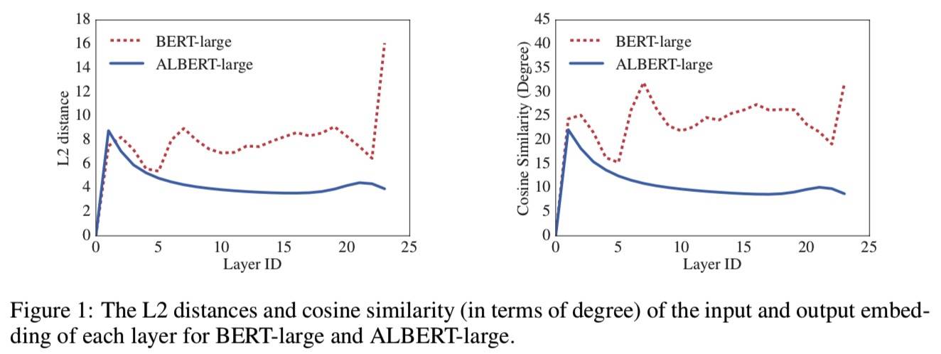
- 跨层共享:共享了层间的所有参数。这里作者对比了 Bert 和 ALBERT 层输入和输出的相似度,发现 ALBERT 的结果更加平滑,说明权重共享对稳定网络参数有影响。另外相似度的结果是振荡的,不是像 DQEs(见《相关工作》)所说的达到了平衡点(对于该平衡点,特定层的输入和输出嵌入保持不变)。
- 句子连贯性损失函数:Bert 的 NSP(Next Sentence Prediction) 被发现不可靠,本文作者猜测任务难度相比 MLM 来说太小,其实它可以看作一个任务做了主题预测和连贯性预测,但主题预测很容易,而且和 MLM 有重叠。因此本文提出了 SOP(Sentence-order Prediction),聚焦在句子连贯的建模上,具体做法是:Positive 和 Bert 一样,来自同一个文档的两个连续片段;Negative 用的还是这两个片段,只不过交换了一下顺序。事实证明 NSP 根本无法解决 SOP 任务(即,它最终学习了更容易的主题预测信号,并在 SOP 任务上以随机基线水平执行),而 SOP 可以将 NSP 任务解决为合理的程度。
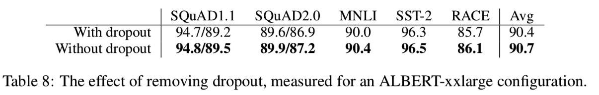
还有个地方要注意,本文并没有使用(其实是在 xxlarge 中)dropout。
接下来是代码部分了,我们直接阅读官方代码(注意,是 1.x 的 Tensorflow,不是最新的 2.x)。模型的整体架构可以简化如下:
1 | class AlbertModel: |
共分为三个组块:Embedding,Transformer 和 Pooling,其中 Embedding 包括了 Token Embedding、Position Embedding 和 Token type Embedding;Transformer 。。。;Pooling 。。。。
Embedding
Token Embedding 比较简单,没有特别的,稍微需要提一下的是 table 的 initializer 都是使用了 tf.truncated_normal_initializer(stddev=0.02),这也包括下面的位置编码和 token type 编码。再就是第一个调整的地方:使用了低维的嵌入(128),后面进到 Transformer 后会先转成 hidden_size。
然后是 Token type Embedding,这里的 type_vocab_size 等于 2,其实就是用 0 和 1 分别表示两个句子,label 就是第二个句子是不是第一个句子的下一句,这是 Bert 的基本配置,参见这里。
接下来是 Position Embedding,使用的是绝对位置编码,先用 max_sequence_len(512)创建一个 table,然后根据 sequence 的长度切片。
此处有感慨,参见《打开脑洞》。
Transformer
首先就是将进来的 Embedding 转为 hidden size(Bert 不需要这一步,因为两者是相等的):
1 | # (batch_size, seq_length, embedding_size) => (batch_size, seq_length, hidden_size) |
然后就是 stack Transformer 了:
1 | for layer_idx in range(num_hidden_layers=12): |
因为这里其实并没有分组(都是 1),所以就是 12 层的 attention_ffn_block stack。看到这里的时候有个关于归一化的疑惑,之前看 Transformer 的时候看的是这个版本:The Annotated Transformer,每个 block 里面是先 norm 再传给 attention layer,出来后和输入做残差连接,当时觉得和图不太一样,也没有多想;后来看到 OpenNMT 也是这么实现的,就更没多想了。但是这次回看了一下 Bert 的代码实现,发现就是和图示一样的:先将输入和 attention layer 的输出做残差连接,再 norm。如果有同学看到这里知道原因的话还希望能告知一二,不胜感激。
接下来看一下 attention_ffn_block:
1 | # 参数都是 base 的 |
这个就是 Transformer(准确来说是 Encoder)的一个 block 了,和原 Bert 的代码对比就可以发现,ALBERT 版本是把 block 单独抽出来作为一个函数(同时也是方便参数共享),另外也把原来的 dense 连接单独抽为一个函数(dense_layer_xd),代码看起来更加清晰。dense_layer_2d 输出的 shape 是 (batch_size, seq_length, hidden_size),而 dense_layer_3d 输出的 shape 则是 (batch_size, seq_length, num_heads, head_size)。
再下来就是 attention layer,也就是 Self attention,Transformer Encoder 的 Attention,qkv 都来自前一层输出的 Attention(可以参考这里的代码):
1 | def attention_layer(from_tensor, |
我们也稍微回顾一下 attention 的计算,之前写过类似的笔记:Bahdanau Attention 和 Luong Attention,另外在 Transformer 笔记中也有介绍过 OpenNMT 的实现,可以参考。下面的实现来自 [Attention is All You Need](Attention Is All You Need Note | Yam)。
1 | def dot_product_attention(q, k, v, mask, dropout_rate=0.1): |
到这里 Transformer 就介绍完了,可以看到虽然源代码量看起来很大,但其实读起来并不复杂,整体还是非常清晰流畅的。
Pooling
这部分非常简单:
1 | first_token_tensor = tf.squeeze(self.sequence_output[:, 0:1, :], axis=1) |
这里的 first_token 其实就是句子标记 CLS,在本模型中就是 0 或 1,0 表示两个句子是连贯的,1 表示两个句子是交换了顺序的,这样做的目的是为了接下来计算 Loss(因为只要 CLS 的结果即可)。
以上就是模型和算法的所有部分了,简单总结一下:
- 模型还是基于 Bert,即 Transformer 的 Encoder 架构。
- 对模型进行了三个调整:分解 Embedding、共享层间参数、SOP 替代 NSP(代码见《如何开始训练》)。
特点和创新
- 分解 Embedding 参数
- SOP 替代 NSP
- 证明 dropout 有损基于 Transformer 的模型
How
如何构造数据
主要的不同是使用了 n-gram masking,也就是随机选择 mask n-gram,n 最大取 3,分布为:
n 为 1 时就是 mask 一个词。
1 | # 取 unigram, bigram, thigram 的概率 |
这段预处理代码比较繁琐,我们稍微简化一下,以词 token 为例:
1 | def create_masked_lm_predictions( |
这里做了不少简化,但足够说明思路了,其实就是根据给定的 p(n) 选择 ngram 作为预测词处理。原代码除了考虑 wordpiece 的情况,还考虑了其他的一些细节,比如不能超过 num_to_predict,不重复处理等等,想起了陈皓的一句话:“细节处尽是魔鬼。”。
最后看一个输入和输出的例子:
1 | print(" ".join(tokens)) |
如何开始训练
这里主要提一下 SOP( Sentence Order Prediction Loss Function),其他的和 Bert 类似,具体原理前面已经提到了,代码如下:
1 | def get_sentence_order_output(pooled_output, labels): |
其实就是个多(二)分类。MLM 的 Loss 不再赘述。
如何使用结果
与 Bert 一样。
数据和实验
层间相似度,对应《模型和算法》的第二个调整:
参数量
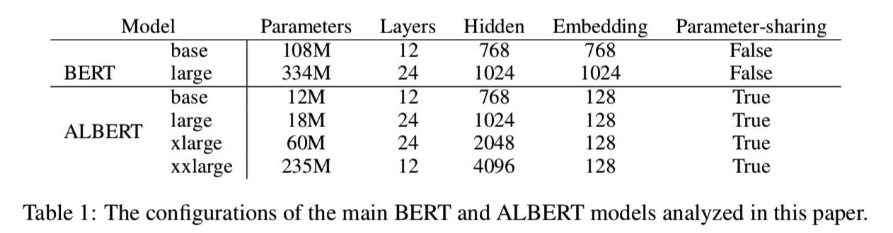
RoBERTa 的参数量在这里,DistilBERT 的参数量是 66M。
Bert vs. ALBERT
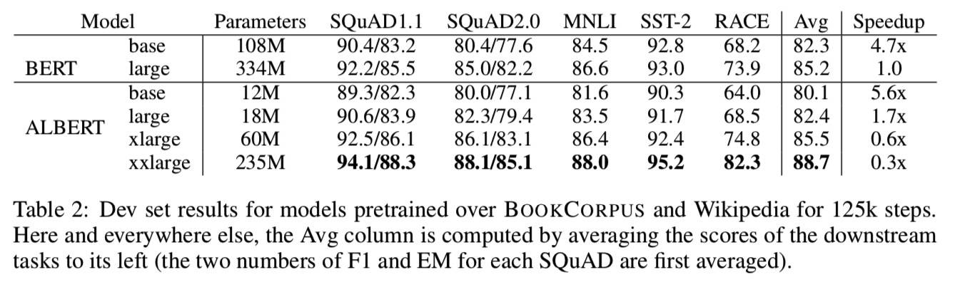
Speedup 是训练时间,以 Bert large 为基准,ALBERT large 速度是 1.7 倍,但 xxlarge 比 Bert large 慢了 3 倍。
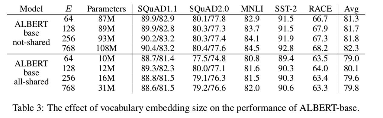
Embedding Size 的影响
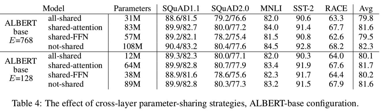
层间参数共享的影响
NSP vs. SOP

Dropout
在各项任务中的表现可以查阅这里。
Discussion
相关工作
扩大语言表征模型
- 语言表征是有用的,近几年最显著的变化是从词或上下文表征到全网络预训练然后下游任务精调。
- 词表征:Tomas Mikolov, Ilya Sutskever, Kai Chen, Greg S Corrado, and Jeff Dean. Distributed represen- tations of words and phrases and their compositionality. In Advances in neural information processing systems, pp. 3111–3119, 2013.
- 句表征:Quoc Le and Tomas Mikolov. Distributed representations of sentences and documents. In Proceedings of the 31st ICML, Beijing, China, 2014.
- 词表征:Jeffrey Pennington, Richard Socher, and Christopher Manning. Glove: Global vectors for word rep- resentation. EMNLP 2014.
- 下游任务:Andrew M Dai and Quoc V Le. Semi-supervised sequence learning. In Advances in neural infor- mation processing systems, pp. 3079–3087, 2015.
- 上下文:Bryan McCann, James Bradbury, Caiming Xiong, and Richard Socher. Learned in translation: Contextualized word vectors. NIPS 2017.
- 上下文:Matthew Peters, Mark Neumann, Mohit Iyyer, Matt Gardner, Christopher Clark, Kenton Lee, and Luke Zettlemoyer. Deep contextualized word representations. ACL 2018.
- 下游任务:Alec Radford, Karthik Narasimhan, Tim Salimans, and Ilya Sutskever. Improving language understanding by generative pre-training. OpenAI, 2018.
- 下游任务:Jacob Devlin, Ming-Wei Chang, Kenton Lee, and Kristina Toutanova. BERT: Pre-training of deep bidirectional transformers for language understanding. ACL 2019.
- 大模型好效果:Alec Radford, Jeffrey Wu, Rewon Child, David Luan, Dario Amodei, and Ilya Sutskever. Language models are unsupervised multitask learners. OpenAI Blog, 1(8), 2019.
- 已有方案:
- 时间换空间:Tianqi Chen, Bing Xu, Chiyuan Zhang, and Carlos Guestrin. Training deep nets with sublinear memory cost. arXiv preprint arXiv:1604.06174, 2016.
- 时间换空间:Aidan N Gomez, Mengye Ren, Raquel Urtasun, and Roger B Grosse. The reversible residual network: Backpropagation without storing activations. In Advances in neural information processing systems, pp. 2214–2224, 2017.
- 并行训练:Colin Raffel, Noam Shazeer, Adam Roberts, Katherine Lee, Sharan Narang, Michael Matena, Yanqi Zhou, Wei Li, and Peter J Liu. Exploring the limits of transfer learning with a unified text-to-text transformer. arXiv preprint arXiv:1910.10683, 2019.
跨层参数共享
关注 Encoder-Decoder 架构:Ashish Vaswani, Noam Shazeer, Niki Parmar, Jakob Uszkoreit, Llion Jones, Aidan N Gomez, Łukasz Kaiser, and Illia Polosukhin. Attention is all you need. In Advances in neural information processing systems, pp. 5998–6008, 2017.
跨层共享效果更好(与本文观察不一致):Mostafa Dehghani, Stephan Gouws, Oriol Vinyals, Jakob Uszkoreit, and Łukasz Kaiser. Universal transformers. arXiv preprint arXiv:1807.03819, 2018.
DQEs,Input 和 Output 能达到平衡点(与本文观察不一致):Shaojie Bai, J. Zico Kolter, and Vladlen Koltun. Deep equilibrium models. In Neural Information Processing Systems (NeurIPS), 2019.
加一个共享参数的 Transformer:Jie Hao, Xing Wang, Baosong Yang, Longyue Wang, Jinfeng Zhang, and Zhaopeng Tu. Modeling recurrence for transformer. Proceedings of the 2019 Conference of the North, 2019.
句子顺序
-
连贯性和衔接性:
- Jerry R. Hobbs. Coherence and coreference. Cognitive Science, 3(1):67–90, 1979.
- M.A.K. Halliday and Ruqaiya Hasan. Cohesion in English. Routledge, 1976.
- Barbara J. Grosz, Aravind K. Joshi, and Scott Weinstein. Centering: A framework for modeling the local coherence of discourse. Computational Linguistics, 21(2):203–225, 1995.
-
用句子预测相邻句子的词:
- Ryan Kiros, Yukun Zhu, Ruslan Salakhutdinov, Richard S. Zemel, Antonio Torralba, Raquel Urtasun, and Sanja Fidler. Skip-thought vectors. NIPS 2015.
- Felix Hill, Kyunghyun Cho, and Anna Korhonen. Learning distributed representations of sentences from unlabelled data. ACL 2016.
-
预测未来的句子:Zhe Gan, Yunchen Pu, Ricardo Henao, Chunyuan Li, Xiaodong He, and Lawrence Carin. Learn- ing generic sentence representations using convolutional neural networks. ACL 2017.
-
预测话语标记:
- Yacine Jernite, Samuel R Bowman, and David Sontag. Discourse-based objectives for fast unsupervised sentence representation learning. arXiv preprint arXiv:1705.00557, 2017.(本文类似)
- Allen Nie, Erin Bennett, and Noah Goodman. DisSent: Learning sentence representations from explicit discourse relations. ACL 2019.
-
预测句对的第二部分是不是被另一个文档的句子替换:Jacob Devlin, Ming-Wei Chang, Kenton Lee, and Kristina Toutanova. BERT: Pre-training of deep bidirectional transformers for language understanding. ACL 2019.(Bert)
-
将预测句子顺序结合在一个三分类任务中:Wei Wang, Bin Bi, Ming Yan, Chen Wu, Zuyi Bao, Liwei Peng, and Luo Si. StructBERT: Incorporating language structures into pre-training for deep language understanding. arXiv preprint arXiv:1908.04577, 2019.
Dropout
CNN 中同时使用批归一化和 dropout 可能导致结果更差:
- Christian Szegedy, Sergey Ioffe, Vincent Vanhoucke, and Alexander A Alemi. Inception-v4, inception-resnet and the impact of residual connections on learning. In Thirty-First AAAI Confer- ence on Artificial Intelligence, 2017.
- Xiang Li, Shuo Chen, Xiaolin Hu, and Jian Yang. Understanding the disharmony between dropout and batch normalization by variance shift. In Proceedings of the IEEE Conference on Computer Vision and Pattern Recognition, pp. 2682–2690, 2019.
加快 ALBERT 的训练和推理速度
- 稀疏注意力:Rewon Child, Scott Gray, Alec Radford, and Ilya Sutskever. Generating long sequences with sparse transformers. arXiv preprint arXiv:1904.10509, 2019.
- 块注意力:Tao Shen, Tianyi Zhou, Guodong Long, Jing Jiang, and Chengqi Zhang. Bi-directional block self- attention for fast and memory-efficient sequence modeling. arXiv preprint arXiv:1804.00857, 2018.
打开脑洞
又到了自由讨论的时间了。首先,必须感慨一下,Google 的代码写的真是实在,很浅白,注释很清楚。记得张俊林老师曾在一篇介绍预训练的知乎文章中评价过 Bert,说它在模型上其实没有太多创新,但是自然、简洁、优雅、有效地解决了问题,我想这可能就是 “工程师” 的 “工程” 两字的价值体现吧。这可能是我们平时应该特别注意和学习的地方,大多数人总是不由自主地把一个别人本来很简洁的东西 “改造” 得很复杂,如果是研究需要,那为了 1-2 个百分点是可以的,但工程上就没太多必要了,那是事倍功半。Google 风格真是越看越爱,导致我现在基本上只跟踪 Google 的最新研究。当然还有个原因——最近这些年 NLP 领域的几个重大突破(Word2Vec,Transformer,Bert)基本都和 Google 有关,这是算法、工程、数据综合后的结果,不应该感到意外。Facebook 则总是会及时做出更加易用和优化的产品(FastText,RoBERTa),当然 Facebook 更强的是推荐和视频领域。由于自己目前做 NLP 工作偏多,自然会更加关注 Google 一些。
然后开始胡侃这篇文章。这篇文章和 Facebook 的 RoBERTa 结果相差不多,但是参数量的确少了不少(毕竟前两个改动都是减少参数的),而且除 xxlarge 外比 DistilBERT 都少(操作起来要比后者省事多了,个人意见,蒸馏真不是一种优雅的方法)。所以实际使用的时候可以酌情考虑 ALBERT 或 RoBERTa,当然对中文来说,考虑到要 wwm(Whole Word Masking),目前开源只有 RoBERTa。
另外有个有意思的地方是 ALBERT 在构造数据时用了 n-gram mask,有点类似 wwm,可以算是一种改进,并没有用 RoBERTa 中的动态 Mask(可能是考虑提升比较微弱吧,但把 NSP 给换成 SOP 了,因为 RoBERTa 证明那没啥用然后就把它给去了),也没有使用 DistilBERT 中的 token prob mask(就是让选择 mask 时更加关注低频词,进而实现对 mask 的平滑取样,我觉得是非常 make sense 的一个点),可能是时间相隔太近吧,看了一下 arxiv 上的第一版的投稿时间,确实只差了 6 天。所以,下一个创新点也许是把这个点加进去?也许说不定已经有了,只是我没关注到。