DistilBERT 论文+代码笔记

Paper:1910.01108.pdf

Code:transformers/examples/distillation at master · huggingface/transformers

核心思想:通过知识蒸馏(在 logits,hidden_states 上计算学生与教师的 loss)训练一个小(主要是层数)模型实现和大模型类似的效果。

What

动机和核心问题

  • 成倍增长的计算成本
  • 模型不断增长的算力和内存要求可能阻止被广泛使用

本文的研究表明,使用经过知识蒸馏得到的的比预训练的小得多的语言模型,可以在许多下游任务上达到类似的性能,而且可以在移动设备上运行。

模型和算法

知识蒸馏 [Bucila 等,2006; Hinton 等,2015] 是一种压缩技术,训练一个紧凑型模型(学生),以再现较大模型(教师)或模型集合的行为。

损失函数

其中,ti 和 si 分别表示老师和学生的概率估计。

使用了 softmax-temperature

其中,T 控制输出分布的平滑程度,推理时设置为 1 变为标准的 Softmax,zi 表示类别 i 的分数。

最终的损失函数是 Lce 和 masked language modeling loss Lmlm 的线性组合,另外作者发现添加余弦嵌入损失(Lcos)有利于使学生和教师隐藏状态向量的方向一致。

学生架构

  • 具有和老师一般的体系结构。
  • 移除了 Token type embedding 和 pooler。
  • 层数减少为 1/2:作者调查发现改变隐层维度对计算效率的影响比其他因素的变化要小(比如层数)。

从老师的两层中选择一层来初始化学生。蒸馏应用了Liu et al. [2019] 提出的 BERT 模型训练最佳实践。语料和 Bert 使用的一致。

蒸馏器代码

我们直接看最核心的代码:

1
2
3
# 一个 batch
token_ids, attn_mask, lm_labels = prepare_batch_mlm(batch=batch)
step(input_ids=token_ids, attention_mask=attn_mask, lm_labels=lm_labels)

无疑,step 就是其核心了,不过在此之前我们先看一下 batch 数据的处理。它 input 的 batch 是一个 tuple,里面包括了 batch_sequence 和 batch_sequence_length,比如其中的一个 batch 结果如下:

1
2
3
4
5
6
7
8
9
10
# batch_size = 2
(tensor([[ 101, 2124, 2004, 15393, 2005, 9167, 1010, 2023, 2152, 1011,
2836, 4800, 1011, 2535, 4337, 2948, 2003, 2881, 3952, 2005,
2250, 19113, 6416, 2007, 3668, 2250, 1011, 2000, 1011, 2598,
3260, 10673, 1012, 102],
[ 101, 2040, 2003, 2183, 2000, 9375, 2129, 3809, 2242, 2038,
2000, 2022, 2077, 8830, 2003, 4072, 1029, 102, 0, 0,
0, 0, 0, 0, 0, 0, 0, 0, 0, 0,
0, 0, 0, 0]]),
tensor([34, 18]))

注意,每次是根据 batch 里的最长序列对其他序列进行 padding 的。

1
2
3
4
5
6
7
8
9
10
11
12
13
14
15
16
17
18
19
20
21
22
23
24
25
26
27
28
29
30
31
32
33
34
35
36
37
38
39
40
41
42
43
44
45
46
47
48
49
50
def prepare_batch_mlm(batch):
token_ids, lengths = batch
# 就是把 padding 部分 mask 掉
# (batch_size, seq_length)
attn_mask = torch.arange(
token_ids.size(1), dtype=torch.long, device=lengths.device) < lengths[:, None]

bs, max_seq_len = token_ids.size()
# 复制 token_ids
mlm_labels = token_ids.new(token_ids.size()).copy_(token_ids)

# 每一个 token_id 的 prob
x_prob = self.token_probs[token_ids.flatten()]
# mlm_mask_prop = 0.15,15% 的 mask
n_tgt = math.ceil(self.mlm_mask_prop * lengths.sum().item())
# 根据大小随机 sample n_tgt 个,不重复取样
tgt_ids = torch.multinomial(x_prob / x_prob.sum(), n_tgt, replacement=False)
# 预测时预测 mask 掉的 15%
pred_mask = torch.zeros(bs * max_seq_len, dtype=torch.bool, device=token_ids.device)
pred_mask[tgt_ids] = 1
pred_mask = pred_mask.view(bs, max_seq_len)
# 让 padding 不参与预测
# 其实这步不需要,因为 token_probs 已经将 padding 的概率设为 0 了,取样是取不到 padding 的
pred_mask[token_ids == self.params.special_tok_ids["pad_token"]] = 0

# 实际要被 mask 掉的 token ids
_token_ids_real = token_ids[pred_mask]
# 从 vocab_size 中随机取出 n_tgt 个 ids
_token_ids_rand = _token_ids_real.clone().random_(self.vocab_size)
# n_tgt 个 mask id
_token_ids_mask = _token_ids_real.clone().fill_(
self.params.special_tok_ids["mask_token"])
# pred_probs = torch.FloatTensor([0.8, 0.1, 0.1])
# 按照 pred_probs 的分布取样 n_tgt 个 => 其中 0 占 80%,1 和 2 接近
probs = torch.multinomial(self.pred_probs, len(_token_ids_real), replacement=True)
# 按照 80%,10%,10% 的分布处理 mask 的 token
# 最终实际为:mask 15%*80%,real 15%*10%,random 15%*10%
_token_ids = (
_token_ids_mask * (probs == 0).long()
+ _token_ids_real * (probs == 1).long()
+ _token_ids_rand * (probs == 2).long()
)
# 用 _token_ids 替换掉原来位置的 token ids
# (batch_size, seq_length)
token_ids = token_ids.masked_scatter(pred_mask, _token_ids)

# label 就是要预测的 mask token,也就是在没有 mask 的位置填充一个负数(不需要预测)
# (batch_size, seq_length)
mlm_labels[~pred_mask] = -100
return token_ids, attn_mask, mlm_labels

这里其实和 Bert 唯一的不同就是 mask 时采用了 token_probs,让选择 mask 时更加关注低频词,进而实现对 mask 的平滑取样(如果按平均分布取样的话,取到的 mask 可能大部分都是重复的高频词)。个人认为这一步还是挺重要的,很 make sense。

现在我们来看 step

1
2
3
4
5
6
7
8
9
10
11
12
13
14
15
16
17
18
19
20
21
22
23
24
25
26
27
28
29
30
31
32
33
34
35
36
37
38
39
40
41
42
43
44
45
46
47
48
49
50
51
52
53
54
55
56
57
58
59
60
61
62
63
64
65
66
67
68
# --alpha_ce 5.0 --alpha_mlm 2.0 --alpha_cos 1.0 --alpha_clm 0.0 --mlm (true)
def step(input_ids, attention_mask, lm_labels):
# 分别计算老师和学生的 logits hidden_states
# (batch_size, seq_lenth, vocab_size)
s_logits, s_hidden_states = \
student(input_ids=input_ids, attention_mask=attention_mask)
with torch.no_grad():
# (batch_size, seq_lenth, vocab_size)
t_logits, t_hidden_states = \
teacher(input_ids=input_ids, attention_mask=attention_mask)

# 计算 mask
if self.params.restrict_ce_to_mask:
# 只计算 mask 的 loss
# (batch_size, seq_lenth, vocab_size)
mask = (lm_labels > -1).unsqueeze(-1).expand_as(s_logits)
else:
# 计算所有 input 不包括 padding 的 mask
# (batch_size, seq_lenth, vocab_size)
mask = attention_mask.unsqueeze(-1).expand_as(s_logits)

# 选择 masked logits
# Returns a new 1-D tensor which indexes the :attr:`input` tensor
# according to the boolean mask :attr:`mask` which is a `BoolTensor`.
s_logits_slct = torch.masked_select(s_logits, mask)
# (n_tgt, vocab_size)
s_logits_slct = s_logits_slct.view(-1, s_logits.size(-1))
t_logits_slct = torch.masked_select(t_logits, mask)
t_logits_slct = t_logits_slct.view(-1, s_logits.size(-1))

# 计算 loss
# temperature = 2.0,推理时为 1.0
# ce_loss_fct = nn.KLDivLoss(reduction="batchmean")
# 定义的损失函数:ti * log(si),计算 KL 散度(衡量两个分步的差异)
loss_ce = self.ce_loss_fct(
F.log_softmax(s_logits_slct / self.temperature, dim=-1),
F.softmax(t_logits_slct / self.temperature, dim=-1)) * (self.temperature) ** 2
# alpha_ce (default 0.5, here 5.0): Linear weight for the distillation loss.
loss = self.alpha_ce * loss_ce

# lm_loss_fct = nn.CrossEntropyLoss(ignore_index=-100)
# (batch_size*seq_length, vocab_size), (batch_size*seq_length, )
loss_mlm = self.lm_loss_fct(s_logits.view(-1, s_logits.size(-1)), lm_labels.view(-1))
# alpha_mlm (default 0.5, here 2.0): Linear weight for the MLM loss
loss += self.alpha_mlm * loss_mlm

# 最后一层的 hidden_state
# (batch_size, seq_length, dim)
s_hidden_states = s_hidden_states[-1]
t_hidden_states = t_hidden_states[-1]
# attention_mask: (batch_size, seq_length), mask: (batch_size, seq_length, dim)
mask = attention_mask.unsqueeze(-1).expand_as(s_hidden_states)
dim = s_hidden_states.size(-1)
s_hidden_states_slct = torch.masked_select(s_hidden_states, mask)
# (sum(lengths), dim)
s_hidden_states_slct = s_hidden_states_slct.view(-1, dim)
t_hidden_states_slct = torch.masked_select(t_hidden_states, mask)
t_hidden_states_slct = t_hidden_states_slct.view(-1, dim)
# (sum(lengths), dim)
target = s_hidden_states_slct.new(s_hidden_states_slct.size(0)).fill_(1)
# cosine_loss_fct = nn.CosineEmbeddingLoss(reduction="mean")
loss_cos = self.cosine_loss_fct(s_hidden_states_slct, t_hidden_states_slct, target)
# alpha_cos (default 0.0, here 1.0): Linear weight of the cosine embedding loss.
loss += self.alpha_cos * loss_cos

# gradient_accumulation_steps (default 50): Gradient accumulation for larger training batches.
loss = loss / self.params.gradient_accumulation_steps
loss.backward()

简单总结一下:

  • 分别计算 teacher 和 student 的 logits 和 hidden_states
  • 计算 mask 的 logits,mask 可以选择只计算 masked tokens,也可以选择计算不含 padding 的 input tokens,两者最后用来计算 loss 的 logits 不相同,其中前者的 size 是 (n_tgt, vocab_size),后者的 size 是 (sum(lenghts), vocab_size)。计算 Lce(散度),并计算 loss:loss = alpha_ce × Lce
  • 直接用 student 的 logits 和 lm_labels 计算 Lmlm(交叉熵),并计算累计 loss:loss += alpha_mlm × Lmlm
  • 计算 mask 的 hidden_states(最后一层),mask 选择不含 padding 的 input tokens(同上面第二种,也是输入的 attention mask),size 为 (sum(lenghts), hidden_dim)。计算 Lcos(余弦嵌入),并计算累计 loss:loss += alpha_cos × Lcos

这样,我们就和前面的理论对应起来了,感性地理解,第一个和第三个 loss 是和教师一致的保证,第二个 loss 是自我(Bert)的保证,非常 make sense。

有两个小地方需要注意一下:

  • MLM 的 labels 是那些 masked 掉的 token_ids(未 mask 的设为一个负数,论文设置为 -100)
  • Cos 的 target 全为 1,size 为 (sum(lengths), )

特点和创新

  • 实践证明了可以通过蒸馏成功地训练通用语言模型。
  • 利用教师的知识进行初始化。
  • 余弦嵌入损失的使用。

How

如何构造数据

根据官方代码文档,准备数据包括两步:

  • binarize the data
  • count the occurrences of each tokens in the data

开始之前首先需要一个 dump.txt,每一行是一个序列,每个序列由几个连贯的句子组成。这个无需再述,我们从 OpenNMT 自带的翻译语料中选择部分作为实验材料。

第一步其实就是对每个序列使用 Bert(或其他)的词表进行 One-Hot 编码,每个文本序列对应一个数组,如:

1
2
3
4
# '[CLS] with the recent plan of ecu 10m, we have slightly enlarged the list of the ngos. [SEP]'
array([ 101, 2007, 1996, 3522, 2933, 1997, 14925, 2226, 2184,
2213, 1010, 2057, 2031, 3621, 11792, 1996, 2862, 1997,
1996, 22165, 1012, 102], dtype=uint16)

第二步是因为使用了 XLM 的 masked language modeling loss 需要平滑 mask token 的分布——更加关注出现次数少的词,所以需要统计数据中 token 的出现次数。最终的结果就是词表中每个 token 的出现次数。

如何开始训练

1
2
3
4
5
6
7
8
9
10
11
12
13
14
15
16
17
18
19
20
21
22
23
24
25
26
27
28
29
30
31
32
33
34
35
36
37
38
39
# From 官方 code
# 指定 student 和 teacher 的类型
student_config_class, student_model_class = DistilBertConfig, DistilBertForMaskedLM
teacher_config_class, teacher_model_class, teacher_tokenizer_class = \
BertConfig, BertForMaskedLM, BertTokenizer

# Tokenizer
tokenizer = BertTokenizer.from_pretrained("bert-base-uncased")

# Data loader,data 和 counts 就是上面得到的两个结果
# mlm_smoothing = 0.7, Smoothing parameter to emphasize more rare tokens
# 因为 1 的 -0.7 次方依然是 1,但是大于 1 的数字就会比 1 小;其实是增加 rare token 的概率
token_probs = np.maximum(counts, 1) ** -mlm_smoothing
for idx in special_tok_ids.values():
token_probs[idx] = 0.0 # do not predict special tokens
token_probs = torch.from_numpy(token_probs)
"""
special_tok_ids =
{'unk_token': 100,
'sep_token': 102,
'pad_token': 0,
'cls_token': 101,
'mask_token': 103}
"""
train_lm_seq_dataset = LmSeqsDataset(params=args, data=data)

# Student
stu_architecture_config = DistilBertConfig.from_pretrained("distilbert-base-uncased.json")
stu_architecture_config.output_hidden_states = True
student = DistilBertForMaskedLM(stu_architecture_config)

# Teacher
teacher = BertForMaskedLM.from_pretrained("bert-base-uncase", output_hidden_states=True)

# Train
distiller = Distiller(
params=args, dataset=train_lm_seq_dataset, token_probs=token_probs,
student=student, teacher=teacher)
distiller.train()

DistilBERT 用的是 Bert 的 Tokenizer,student 和 teacher 分别是两个对应的 MaskedLM。

如何使用结果

与 Bert 一样。

数据和实验

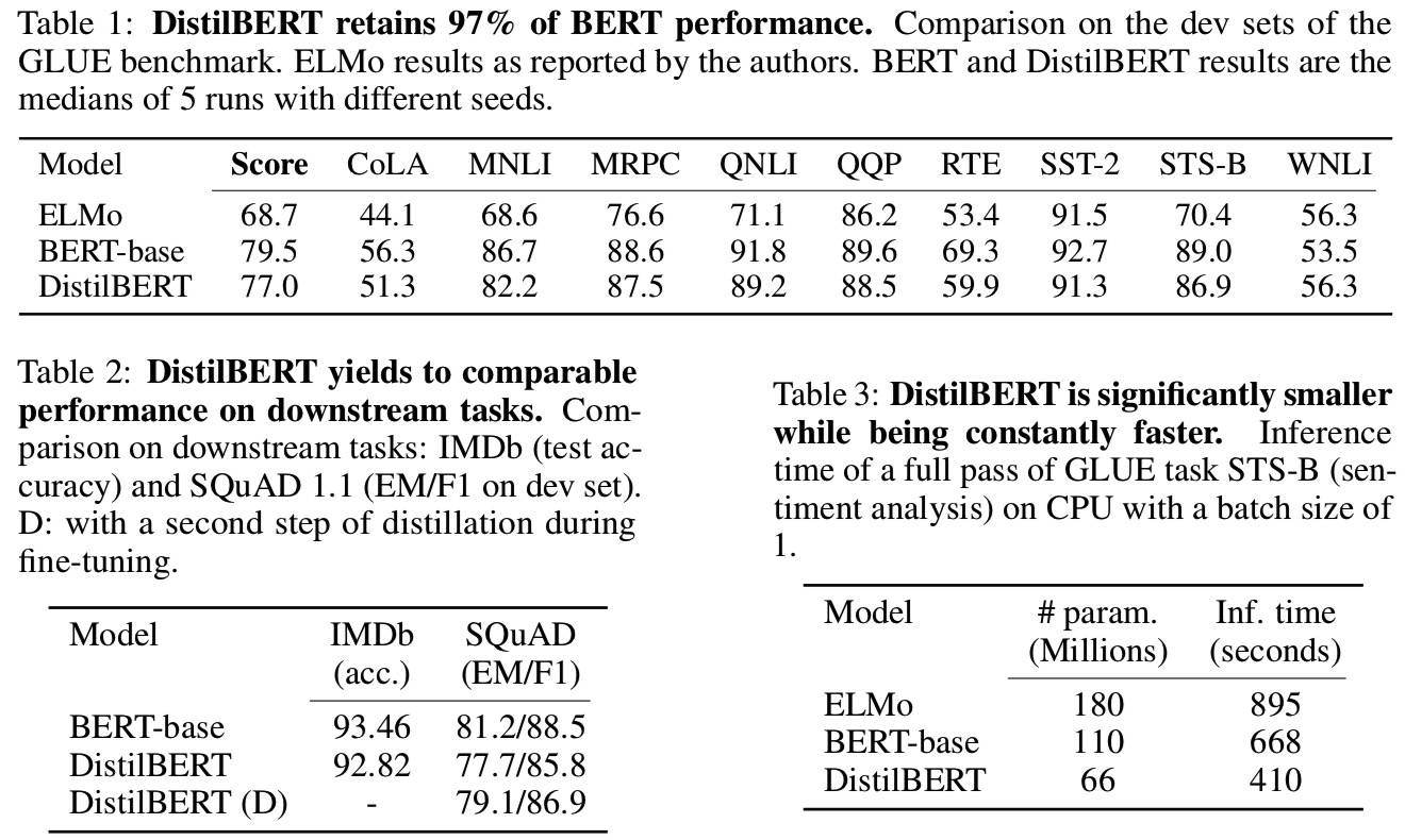
40% smaller, 60% faster, that retains 97% of the language understanding capabilities.

Discussion

相关工作

Task-specific distillation

  • 将精调的分类模型 BERT 转移到基于 LSTM 的分类器:Raphael Tang, Yao Lu, Linqing Liu, Lili Mou, Olga Vechtomova, and Jimmy Lin. Distilling task-specific knowledge from bert into simple neural networks. ArXiv, abs/1903.12136, 2019.
  • 由 BERT 初始化较小的 Transformer 模型,在 SQuAD 上精调:Debajyoti Chatterjee. Making neural machine reading comprehension faster. ArXiv, abs/1904.00796, 2019.
  • 使用原始的预训练目标来训练较小的学生,然后通过蒸馏进行精调:Iulia Turc, Ming-Wei Chang, Kenton Lee, and Kristina Toutanova. Well-read students learn better: The impact of student initialization on knowledge distillation. ArXiv, abs/1908.08962, 2019.

Multi-distillation

  • 多任务:Ze Yang, Linjun Shou, Ming Gong, Wutao Lin, and Daxin Jiang. Model compression with multi-task knowledge distillation for web-scale question answering system. ArXiv, abs/1904.09636, 2019.
  • 多语言:Henry Tsai, Jason Riesa, Melvin Johnson, Naveen Arivazhagan, Xin Li, and Amelia Archer. Small and practical bert models for sequence labeling. In EMNLP-IJCNLP, 2019.

Other compression techniques

  • 剪枝:Paul Michel, Omer Levy, and Graham Neubig. Are sixteen heads really better than one? In NeurIPS, 2019.
  • 量化:Suyog Gupta, Ankur Agrawal, Kailash Gopalakrishnan, and Pritish Narayanan. Deep learning with limited numerical precision. In ICML, 2015.