Logistic Regression Note (SLP Ch05)

In NLP, logistic regression is the baseline supervised machine learning algorithm for classification.

discriminative classifier: like logistic regression
- only trying to learn to distinguish the classes.
- directly compute $P(c|d)$
generative classifier: like naive Bayes
- have the goal of understanding what each class looks like.
- makes use of likelihood term $P(d|c)P(c)$

A machine learning system for classification has four components:

A feature representation of the input
A classification function that computes $\hat y$ , the estimated class, via $p(y|x)$ . Like sigmoid and softmax.
An objective function for learning, usually involving minimizing error on training examples. Like cross-entropy loss function.
An algorithm for optimizing the objective function. Like stochastic gradient descent.

Classification: the sigmoid

Logistic regression solves task by learning from a training set, a vector of weights and a bias term (also called intercept).

$z = w · b$ $y = \sigma(z) = \frac {1}{1 + e^{-z}}$ $P(y=1) = \sigma(w·x+b) = \frac{1}{1+e^{-(w·x+b)}}$ $P(y=0) = 1- \sigma(w·x+b) = 1 - \frac{1}{1+e^{-(w·x+b)}} = \frac{e^{-(w·x+b)}}{1+e^{-(w·x+b)}}$

decision boundary:

y^ = 1 if P(y=1|x) > 0.5, otherwise = 0

Designing features: Features are generally designed by examining the training set with an eye to linguistic intuitions and the linguistic literature on the domain. For logistic regression and naive Bayes combination features or feature interactions have to be designed by hand.

For many tasks we’ll need large numbers of features, they are created automatically via feature templates, abstract specifications of features.

In order to avoid the extensive human effort of feature design, recent research in NLP has focused on representation learning: ways to learn features automatically in an unsupervised way from the input.

Choosing a classifier: Naive Bayes has overly strong conditional independence assumptions. If two features are strongly correlated, naive Bayes will overestimate the evidence.

Logistic regression generally works better on larger documents or datasets and is a common default.
Naive Bayes works extremely well on very small datasets or short documents, also easy to implement and very fast to train.

Learning in Logistic Regression

The distance between system output and gold output is called loss function or cost function.
Need an optimization algorithm for iteratively updating the weights so as to minimize the loss function.

The cross-entropy loss function

L(y^, y) = How much y^ differs from the true y

MSE loss: $L_{MSE}(\hat y, y) = \frac{1}{2} (\hat y -y)^2$

It’s useful for some algorithms like linear regression, but becomes harder to optimize (non-convex) when it’s applied to probabilistic classification.

Instead, we use a loss function that prefers the correct class labels of the training example to be more likely. This is called conditional maximum likelihood estimation: we choose the parameters w,b that maximize the log probability of the true y labels in the training data given the observations x. The resulting loss function is the negative log likelihood loss, generally called the cross entropy loss.

We’d like to learn weights that maximize the probability of the correct label p(y|x). Since there are only two discrete outcomes (1 or 0):

$p(y|x) = \hat y^y (1-\hat y)^{1-y}$ $\log p(y|x) = y \log \hat y + (1-y) \log (1-\hat y)$ $L_{CE}(\hat y, y) = -\log p(y|x) = -[y \log \hat y + (1-y) \log (1-\hat y)]$ $L_{CE}(w, b) = -[y \log \sigma(w·x+b) + (1-y) \log (1-\sigma(w·x+b))]$

A perfect classifier would assign probability 1 to the correct outcome (y=1 or y=0) and probability 0 to the incorrect outcome. That means the higher ˆy (the closer it is to 1), the better the classifier; the lower ˆy is (the closer it is to 0), the worse the classifier. The negative log of this probability is a convenient loss metric since it goes from 0 (negative log of 1, no loss) to infinity (negative log of 0, infinite loss).

This loss function also insures that as probability of the correct answer is maximized, the probability of the incorrect answer is minimized; since the two sum to one, any increase in the probability of the correct answer is coming at the expense of the incorrect answer.

We make the assumption that the training examples are independent:

$\log p(training\ labels) = \log \prod_{i-1}^m p(y^{(i)} |x^{(i)}) = \sum_{i=1}^m \log p(y^{(i)} |x^{(i)}) = -\sum_{i=1}^m L_{CE} (\hat y^{(i)} ,y^{(i)})$ $Cost(w,b) = \frac{1}{m} \sum_{i=1}^m L_{CE} (\hat y^{(i)}, y^{(i)}) = -\frac{1}{m} \sum_{i=1}^m y^{(i)} \log \sigma(w·x^{(i)}+b) + (1-y^{(i)}) \log (1-\sigma(w·x^{(i)}+b))$

Gradient Descent

$\hat \theta = \arg \min_\theta \frac{1}{m} \sum_{i=1}^m L_{CE} (y^{(i)}, x^{(i)};\theta)$

Gradient descent is a method that finds a minimum of a function by figuring out in which direction
(in the space of the parameters θ) the function’s slope is rising the most steeply, and moving in the opposite direction.

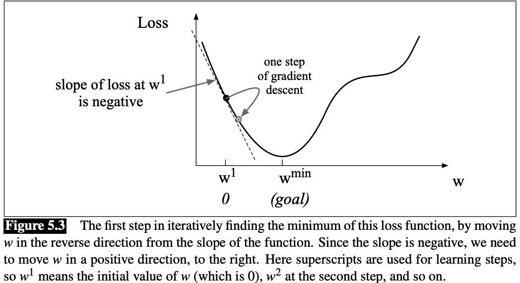
The magnitude of the amount to move in gradient descent is the value of the slope d/dw f(x;w) weighted by a learning rate η:

$w^{t+1} = w^t - \eta \frac {d}{dw} f(x;w)$ $\nabla_\theta L(f(x;\theta),y)) = \frac{\partial}{\partial W} L(f(x;\theta),y)$ $\theta_{t+1} = \theta_t - \eta \nabla L(f(x;\theta),y)$

The Gradient for Logistic Regression

$\frac{\partial L_{CE} (w,b)}{\partial w_j} = [\sigma(w·x+b)-y]x_j$ $\frac{\partial Cost(w,b)}{\partial w_j} = \sum_{i=1}^m [\sigma(w·x^{(i)} +b) - y^{(i)}]x_j^{(i)}$

The Stochastic Gradient Descent Algorithm

function STOCHASTIC GRADIENT DESCENT (L(), f(), x, y) returns θ
θ ← 0
repeat T times
	For each training tuple(xi, yi) (random order)
    Compute y^i = f(xi; θ) # estimated output y^
    # Compute loss L(y^i, yi) # how far y^i from true output yi
    g←▽θ L(f(xi;θ), yi) # gradient
    θ←θ-ηg # how to move θ to minimize loss
return θ

The code is here: Stochastic-Gradient-Descent

Regularization

If the weights for features fit too perfectly, noisy factors just accidentally correlate with the class. This problem is overfitting. To avoid overfitting, a regularization term is added to the objective function:

$\hat w = \arg \max_w \sum_{i=1}^m \log P(y{(i)}|x^{(i)}) - \alpha R(w)$

R(w) is used to penalize large weights. There are two common regularization terms R(w):

L2 regularization, also called ridge:
- easier to optimize because of simple derivative
- prefers weight vectors with many small weights
- α = λ/2m
L1 regularization, also called lasso:
- more complex because the derivative of |w| is non-continuous at zero
- prefers sparse solutions with some larger weights but many more weights set to zero
- α = λ/m

Both L1 and L2 regularization have Bayesian interpretations as constraints on the prior of how weights should look.

L1 can be viewed as a Laplace prior on the weights
L2 corresponds to assuming that weights are distributed according to a gaussian distribution with mean is 0

Multinomial logistic regression

Use multi-nominal logistic regression, also called softmax regression.

$softmax(z_i) = \frac{e^{z_i}} {\sum_{j=1}^k e^{z_j}} \ 1≤i≤k$

Σ is used to normalize all the values into probabilities.

$p(y=c|x) = \frac{e^{w_c · x + b_c}} {\sum_{j=1}^k e^{w_j · x + b_j}}$

Features in Multinomial Logistic Regression

A feature might have a negative weight for 0 documents, and a positive weight for + or - documents.

Learning in Multinomial Logistic Regression

$L_{CE}(\hat y, y) = -\sum_{k=1}^K 1 \{y=k\} \log p(y=k|x) = -\sum_{k=1}^K 1 \{y=k\} \log \frac {e^{w_k · x + b_k}} {\sum_{j=1}^k e^{w_j · x + b_j}}$

The gradient is:

$\frac {\partial L_{CE}}{ \partial w_k} = (1 \{y=k\} - p(y=k|x)) x_k = (1\{y=k\} - \frac {e^{w_k · x + b_k}} {\sum_{j=1}^k e^{w_j · x + b_j}} ) x_k$

Interpreting models

Logistic regression can be combined with statistical tests (the likelihood ratio test, or the Wald test); investigating whether a particular feature is significant by one of these tests, or inspecting its magnitude (how large is the weight w associated with the feature?) can help us interpret why the classifier made the
decision it makes. This is enormously important for building transparent models.

Summary

Logistic regression is a supervised machine learning classifier that extracts real-valued features from the input, multiplies each by a weight, sums them, and passes the sum through a sigmoid function to generate a probability. A threshold is used to make a decision.
Logistic regression can be used with two classes or with multiple classes (use softmax to compute probabilities).
The weights (vector w and bias b) are learned from a labeled training set via a loss function, such as the cross-entropy loss, that must be minimized.
Minimizing this loss function is a convex optimization problem, and iterative algorithms like gradient descent are used to find the optimal weights.
Regularization is used to avoid overfitting.
Logistic regression is also one of the most useful analytic tools, because of its ability to transparently study the importance of individual features.

Yam

Feeling, Coding, Thinking