说明:来自卷积神经网络 - 网易云课堂的关键点记录,用来随时查阅,多图(88张)。课程真的很好;)
目录
Week1 卷积神经网络
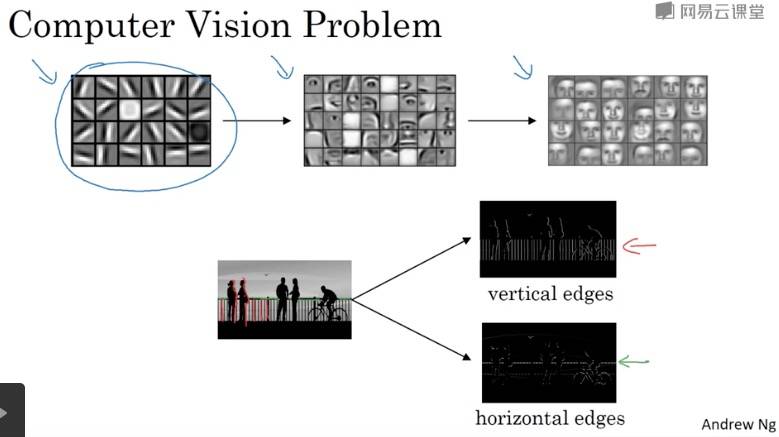
计算机视觉
Why CNN?
因为普通网络参数太多,比如 1000×1000 的图片,输入的维度为 1000×1000×3 = 3 million,假设全连接层的下一层为 1000 个节点,那么第一层的 W 矩阵将大小为:(1000, 3m),也就是有 3 billion 个参数。
边缘检测示例
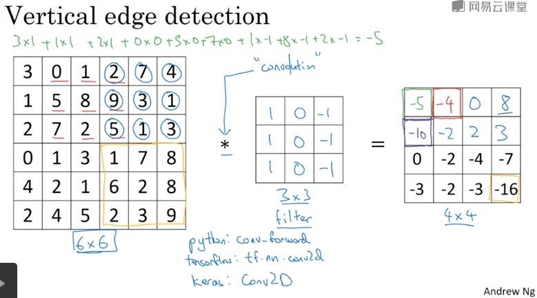
Question: 滤波器(kernel)的选择标准是什么?(下一节会涉及)

检测到的垂直边缘看起来很粗,是因为图片本身很小。
例子中 kernel 表示:左边是明亮的像素,右边是深色的像素。
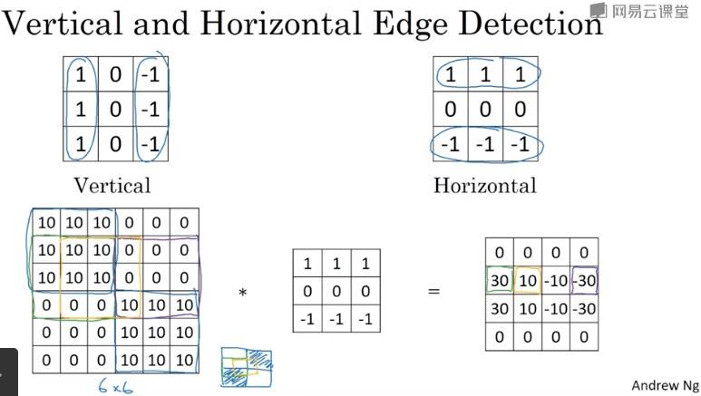
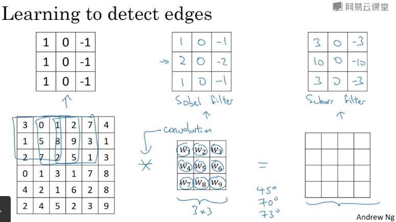
更多边缘检测内容

Padding
刚刚的做法有两个缺点:
- 每次图片会缩小,如 6×6 → 4×4
- 边上的像素点只被一个输出所触碰或者说使用,意味着丢掉了边缘的部分信息
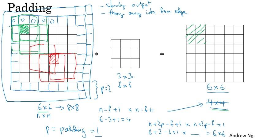
那么到底要填充多少像素:
- Valid: No Padding
- Same: InputSize == OutputSize, 与过滤器有关,过滤器的大小一般都是奇数
- 如果是偶数,因为 pading = (filter-1)/2,所以只能使用一些不对称填充
- 奇数过滤器有一个中心点,便于指出过滤器的位置(计算机视觉的惯例)

卷积步长
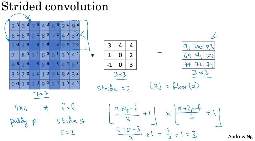
惯例:采用地板除,即只要过滤器超出矩阵,就不再计算。
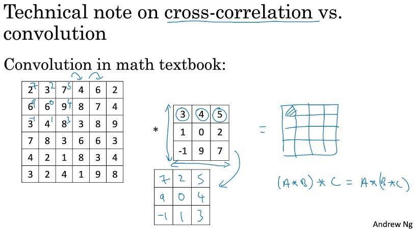
按照机器学习的惯例,通常不进行翻转操作,从技术上说,这个操作可能叫做互相关更好。但在大部分深度学习文献中都把它叫做卷积运算。信号处理或某些数学运算中,卷积的定义包含翻转。
卷积为何有效
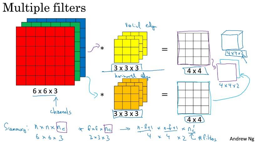
输入的 channel 必须与 filter 的 channel 相等。
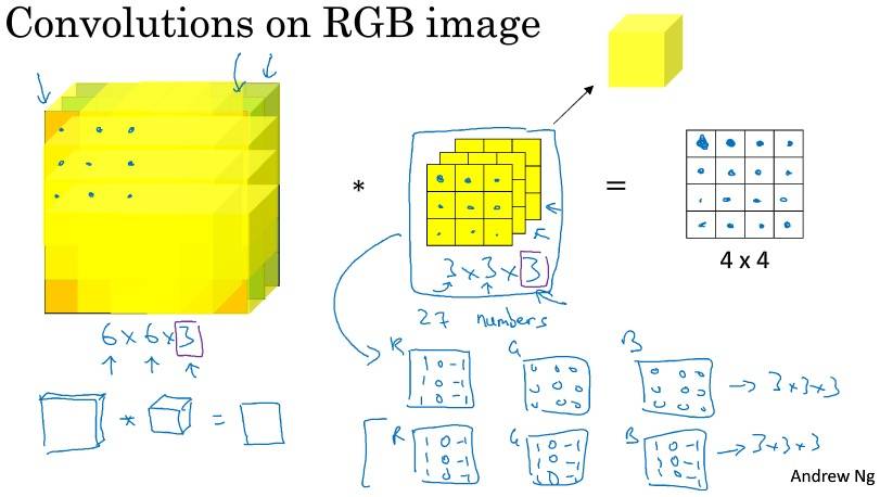
多个过滤器,输出通道等于要检测的特征数(过滤器就可看作特征)。
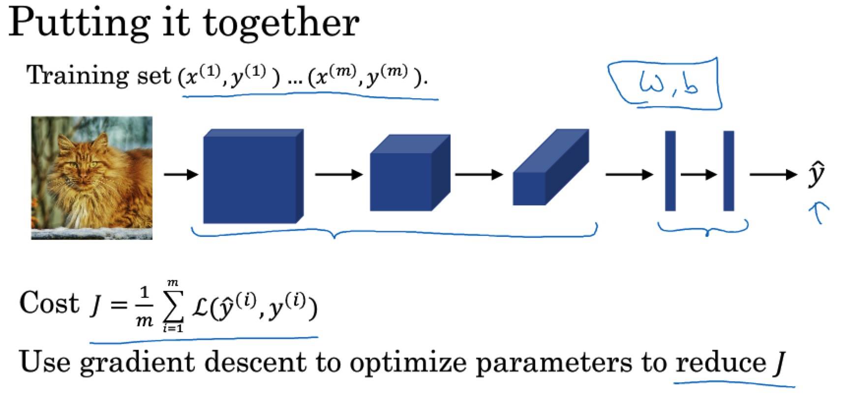
单层卷积网络

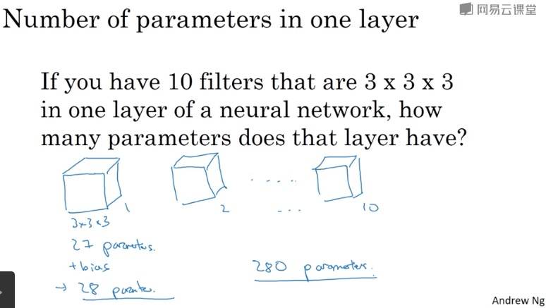
无论输入大小如何,参数和过滤器有关(保持不变),这是卷积神经网络的一个特征:“避免过拟合”。

简单卷积网络示例
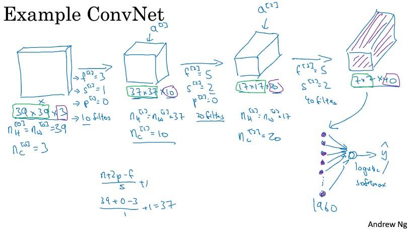
卷积网络随着深度增加:宽度和高度在一段时间内不变,然后减小;信道数量在增加。
Types of layer in a convolutional network:
- Convolution
- Pooling
- Fully connected
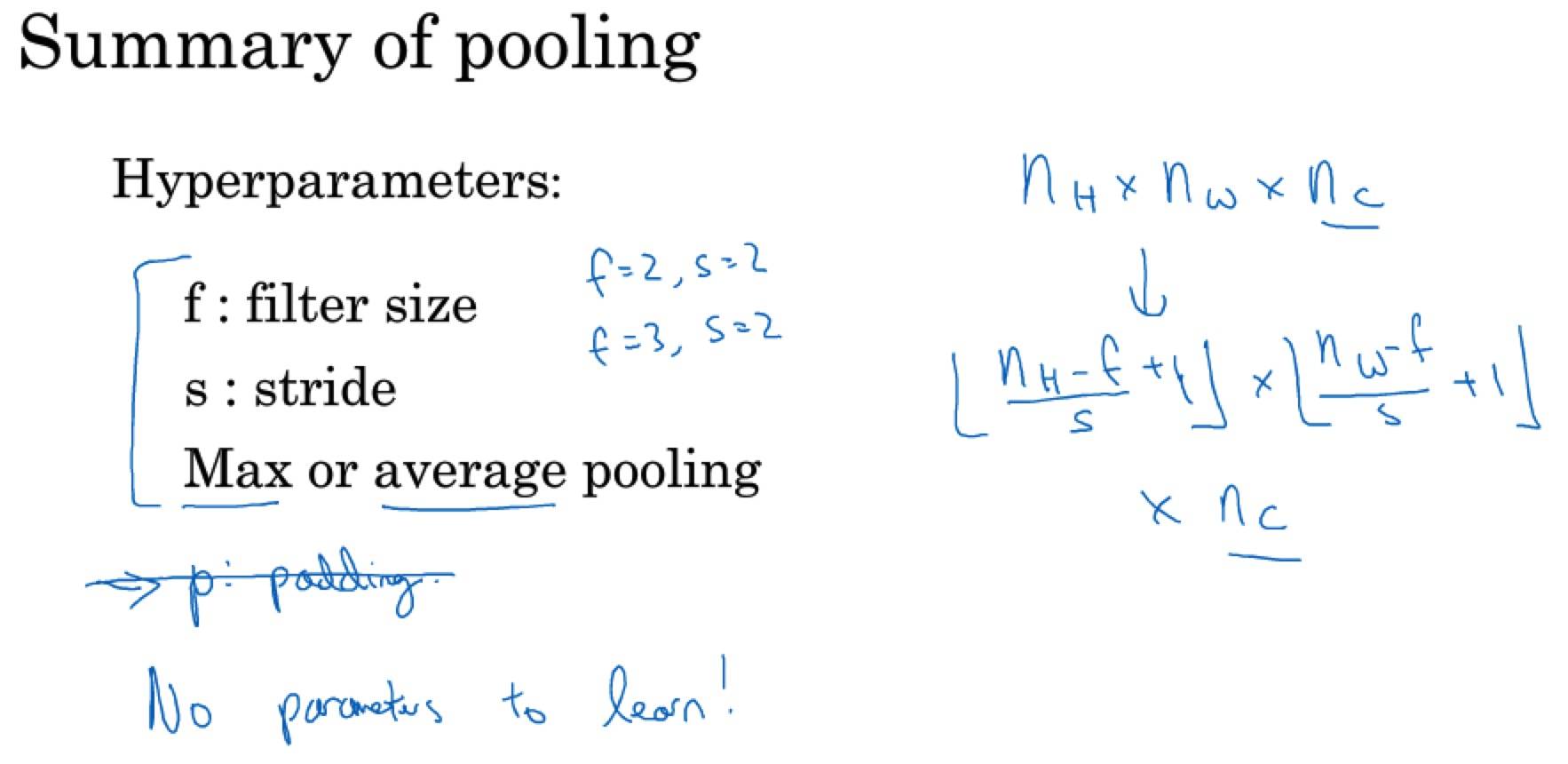
池化层
有一组超参数,并没有参数需要学习。
最大池化算法:取过滤器选中的矩阵中的最大值;平均池化:取平均值,不太常用(深度很深时会用到)。
f=2, s=2 其效果相当于表示层的高度和宽度缩减一半。
大部分情况下,最大池化很少用到 padding。
卷积神经网络示例
随着神经网络深度的加深,高度 nH 和宽度 nW 通常都会减少,信道数量会增加。

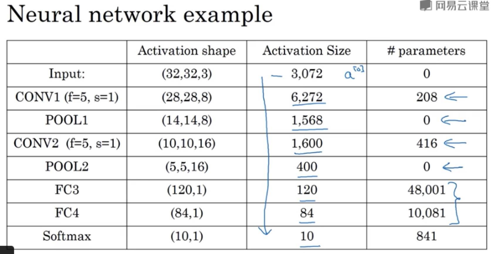
208 = 5*5*8 + 8416 = 5*5*16 + 1648001 = 400*120 + 110081 = 120*84 + 1841 = 84*10 + 1- 后面加的是偏置参数
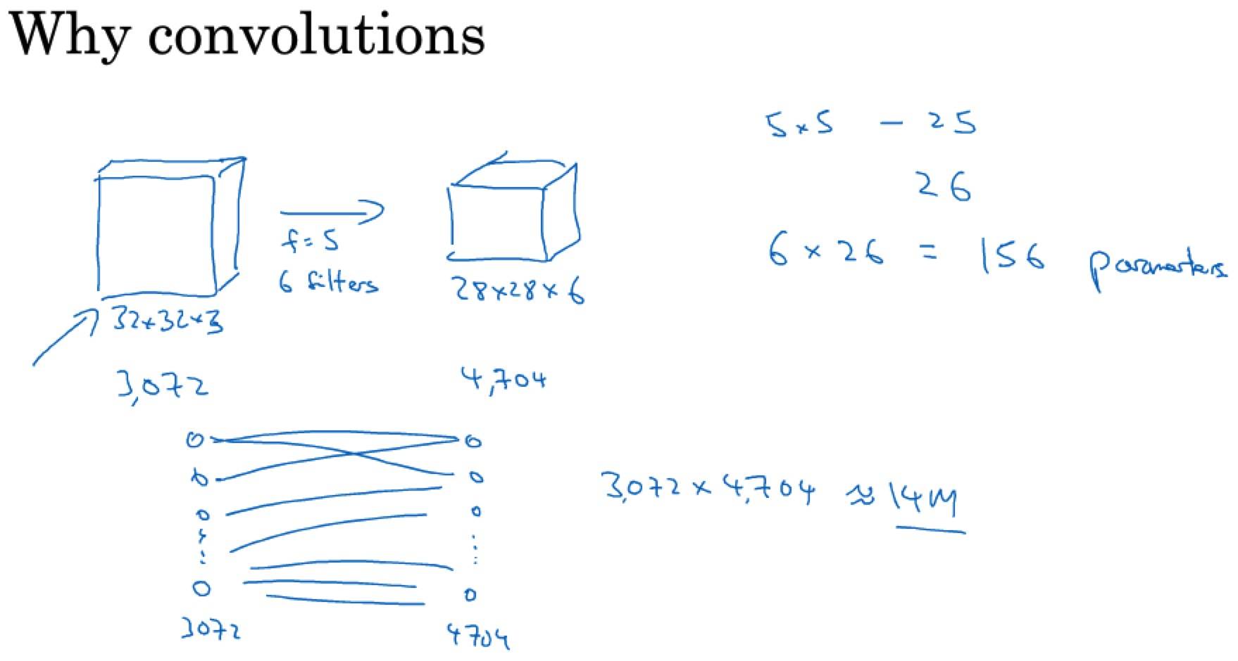
为什么使用卷积?
与只用全连接层相比,卷积层的两个优势在于:
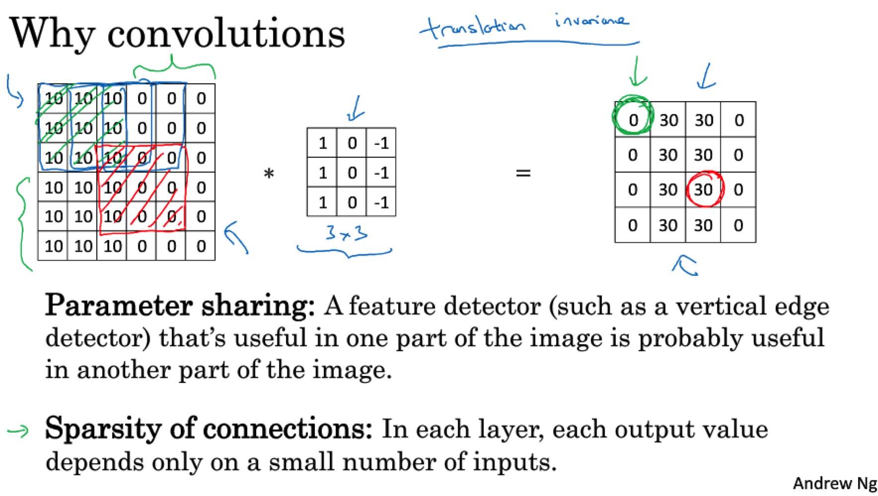
- 参数共享
- 稀疏连接
善于捕捉平移不变:图像平移几个像素,不会发生太大改变,卷积结构使得即使移动几个像素,图片依然具有非常相似的特征,应该属于同样的输出标记。
注意点&Tips
- 上一层的每个过滤器结果叠加后才是这一层一个过滤器的结果。
- 对叠加后的结果 Pooling,这一层有多少个过滤器,就 Pooling 多少次。
Week2 深度卷积网络:实例探究
为什么要进行实例探究?
架构往往是通用的。
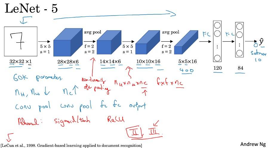
经典网络
LeNet-5 Sigmoid 和 Tanh 激活函数;每个过滤器和输入模块信道数量相同;池化后非线性处理。
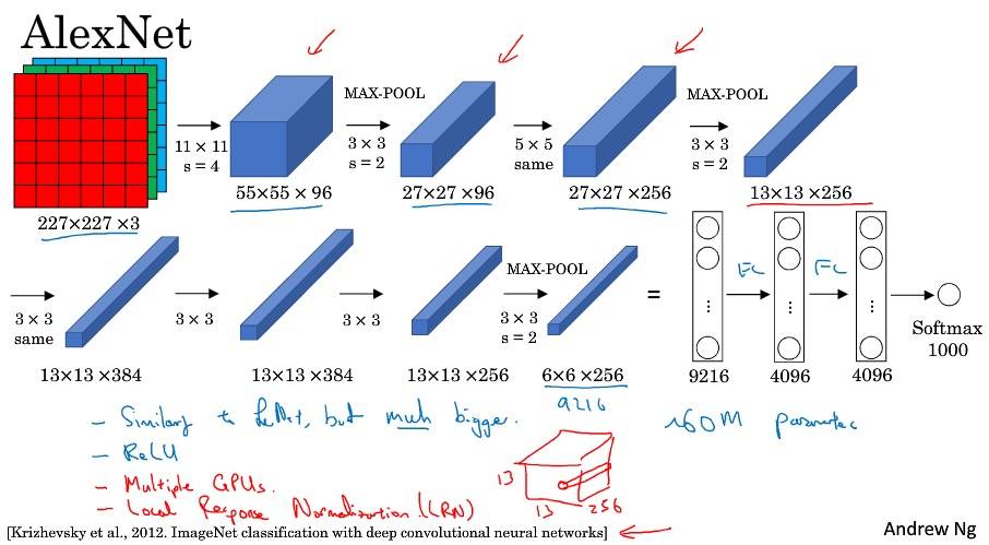
AlexNet 比 LeNet 大很多(60 million 参数);使用了 ReLU 激活函数;多 GPU;LRN(局部响应归一化)。
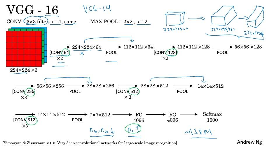
VGG-16 简化了神经网络结构;特征数量巨大(138 million 参数)。
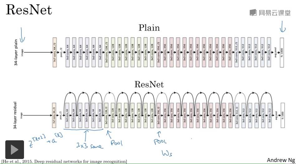
残差网络
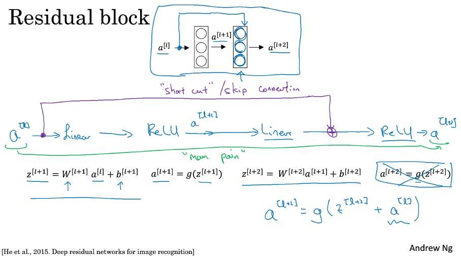
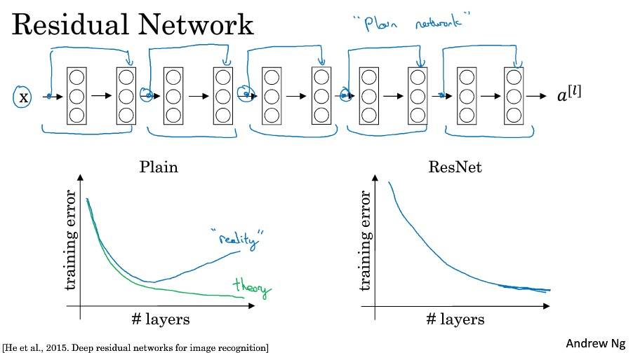
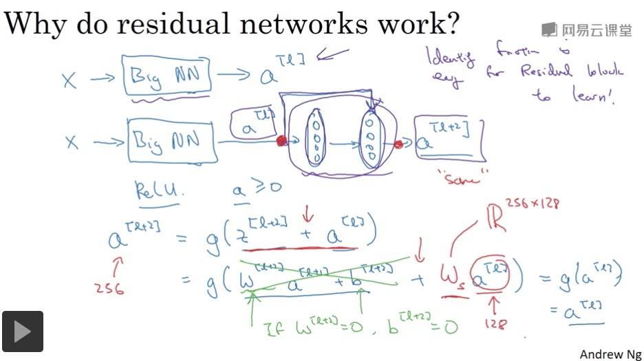
残差网络为什么有用?
残差块学习恒等函数非常容易,不会降低网络性能。
ResNets 使用了许多相同卷积,所以 a[l] 的维度等于输出层的维度,从而实现了跳远连接。
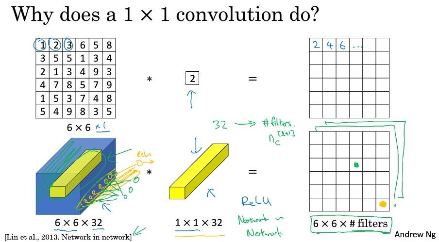
网络中的网络以及 1×1 卷积
可以理解为所有单元都应用了一个全连接神经网络。
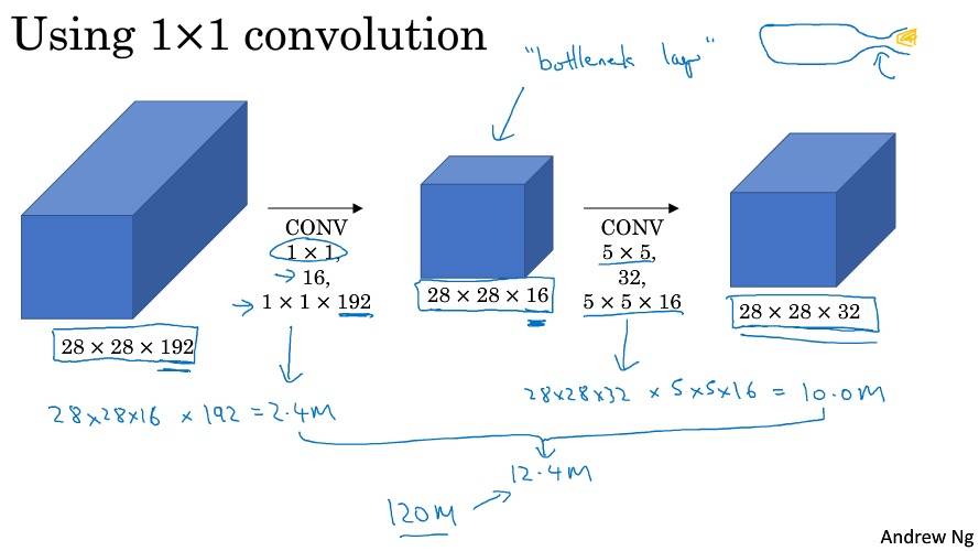
可以通过 1×1 卷积的简单操作来压缩、保持甚至增加输入层中的信道数量。

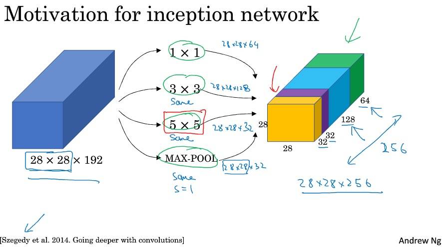
Google Inception 网络简介
Inception 网络不需要人为决定使用哪个过滤器。

Inception 网络
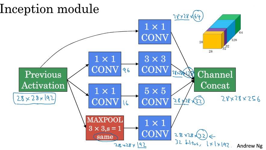
分支,通过隐层做出预测,起到调整效果,并防止过拟合。GoogLeNet。

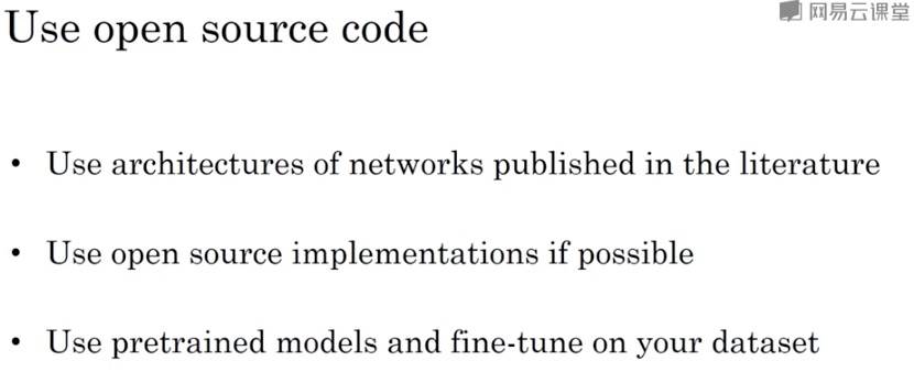
使用开源的实现方案
先选择一个喜欢的框架,找一个开源实现,在此基础上进行开发。
迁移学习
- 如果数据集比较小
- 通过深度学习框架的参数固定已经训练的层,让其不参与训练
- 最后一个隐层的特征结果存到硬盘,直接用此结果连接 softmax 进行训练
- 如果数据集比较大
- 冻结更少的层
- 如果有大量数据
- 训练整个网络(用作者的参数初始化,代替随机初始化)

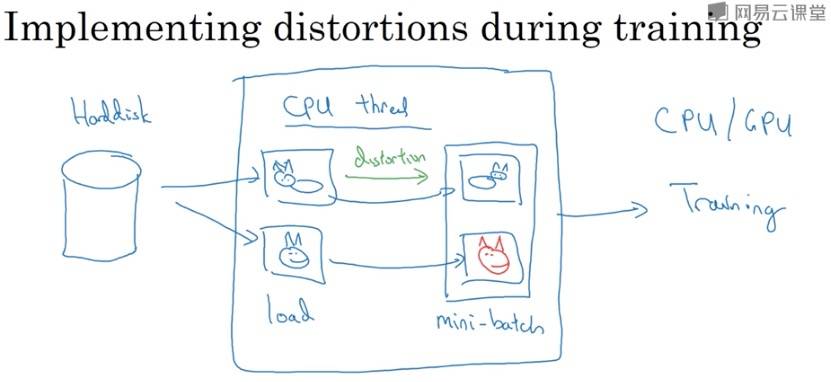
数据扩充
计算机视觉一个主要问题是没有办法得到充足的数据,所以数据增强很有必要。
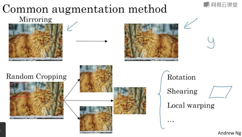

在实践中,RGB 的值是根据某种概率分布来决定的。
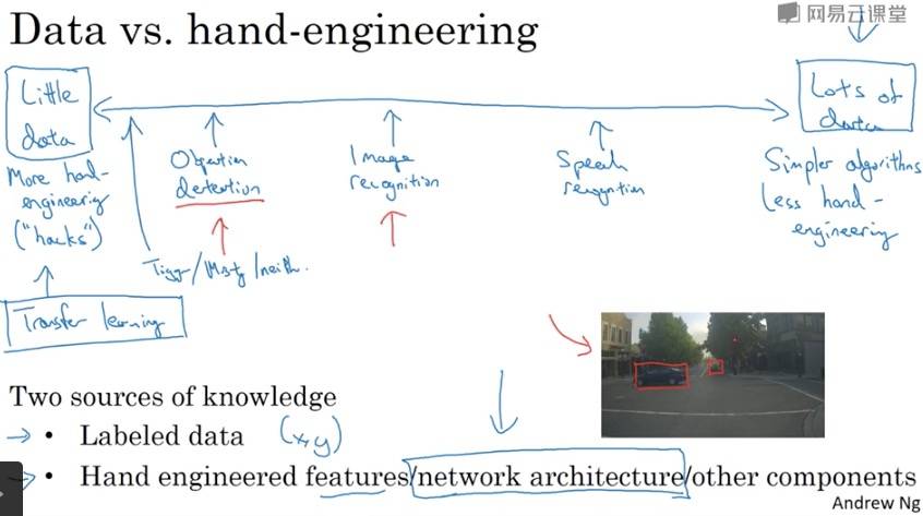
计算机视觉现状
当有很多数据时,人们倾向于使用更简单的算法和更少的手工工程。相反则有更多的手工工程。
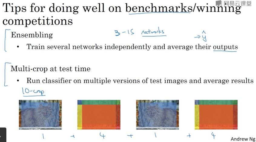
集成,即已有的模型。
注意点&Tips
-
If you have not yet achieved a very good accuracy (let’s say more than 80%), here’re some things you can play around with to try to achieve it:
- Try using blocks of CONV->BATCHNORM->RELU such as:
1
2
3
4
5
6
7
8
9
X_input = Input(input_shape)
X = ZeroPadding2D((3, 3))(X_input)
X = Conv2D(32, (3, 3), strides = (1, 1), name = 'conv0')(X)
X = BatchNormalization(axis = 3, name = 'bn0')(X)
X = Activation('relu')(X)
X = MaxPooling2D((2,2), name='max_pool')(X)
X = Flatten()(X)
X = Dense(1, activation='sigmoid', name='fc')(X)
model = Model(inputs=X_input, outputs=X, name='HappyModel')
until your height and width dimensions are quite low and your number of channels quite large (≈32 for example). You are encoding useful information in a volume with a lot of channels. You can then flatten the volume and use a fully-connected layer.
- You can use MAXPOOL after such blocks. It will help you lower the dimension in height and width.
- Change your optimizer. We find Adam works well.
- If the model is struggling to run and you get memory issues, lower your batch_size (12 is usually a good compromise)
- Run on more epochs, until you see the train accuracy plateauing.
- Try using blocks of CONV->BATCHNORM->RELU such as:
-
Create->Compile->Fit/Train->Evaluate/Test.
1
2
3
4
happyModel = HappyModel(X_train[0].shape)
happyModel.compile(optimizer='Adam', loss='binary_crossentropy', metrics=['accuracy'])
happyModel.fit(x=X_train, y=Y_train, epochs=50, batch_size=12)
preds = happyModel.evaluate(x=X_test, y=Y_test) -
other basic features of Keras
1
2
3
happyModel.summary()
plot_model(happyModel, to_file='HappyModel.png')
SVG(model_to_dot(happyModel).create(prog='dot', format='svg')) -
Identify block
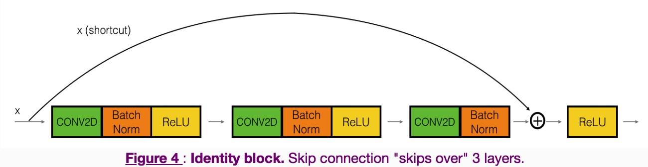
-
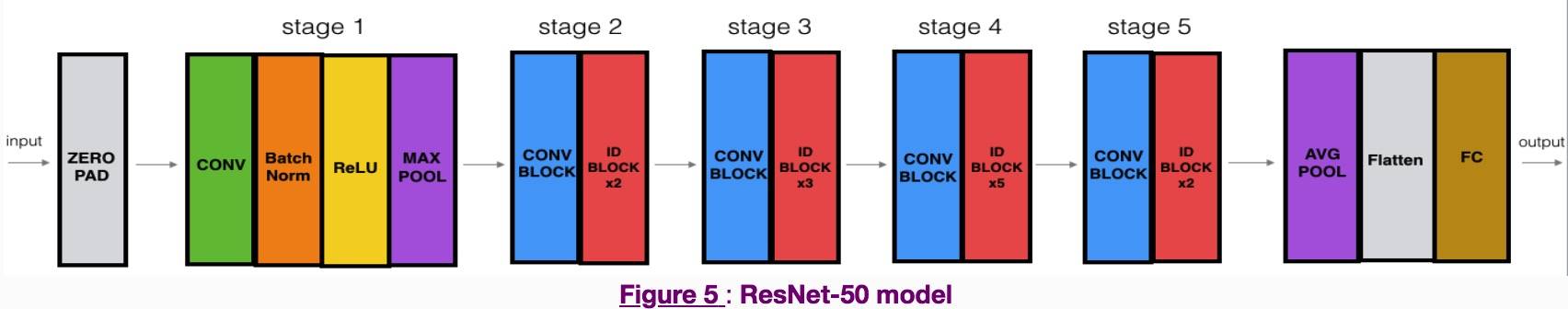
Convolutional block

-
ResNet model
Week3 目标检测
目标定位


一般情况下的损失函数:
- 分类:对数损失函数
- 坐标:平方误差
- 对象:逻辑回归
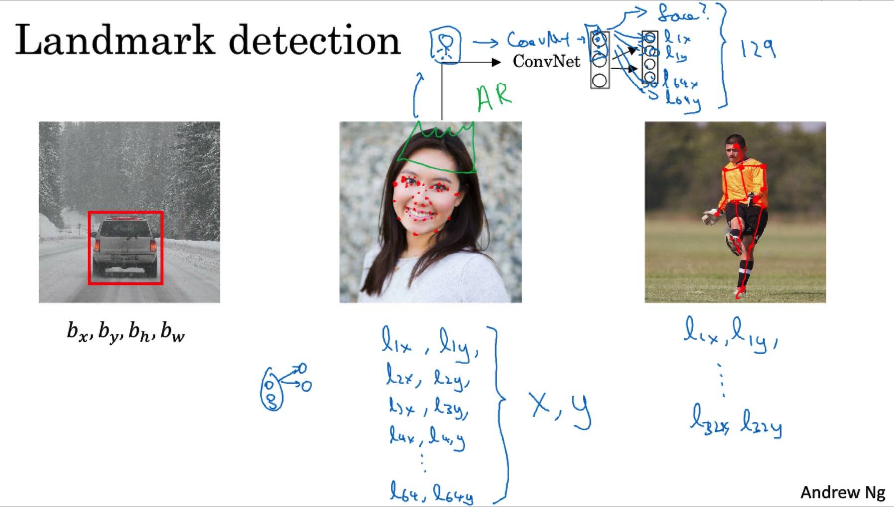
特征点监测
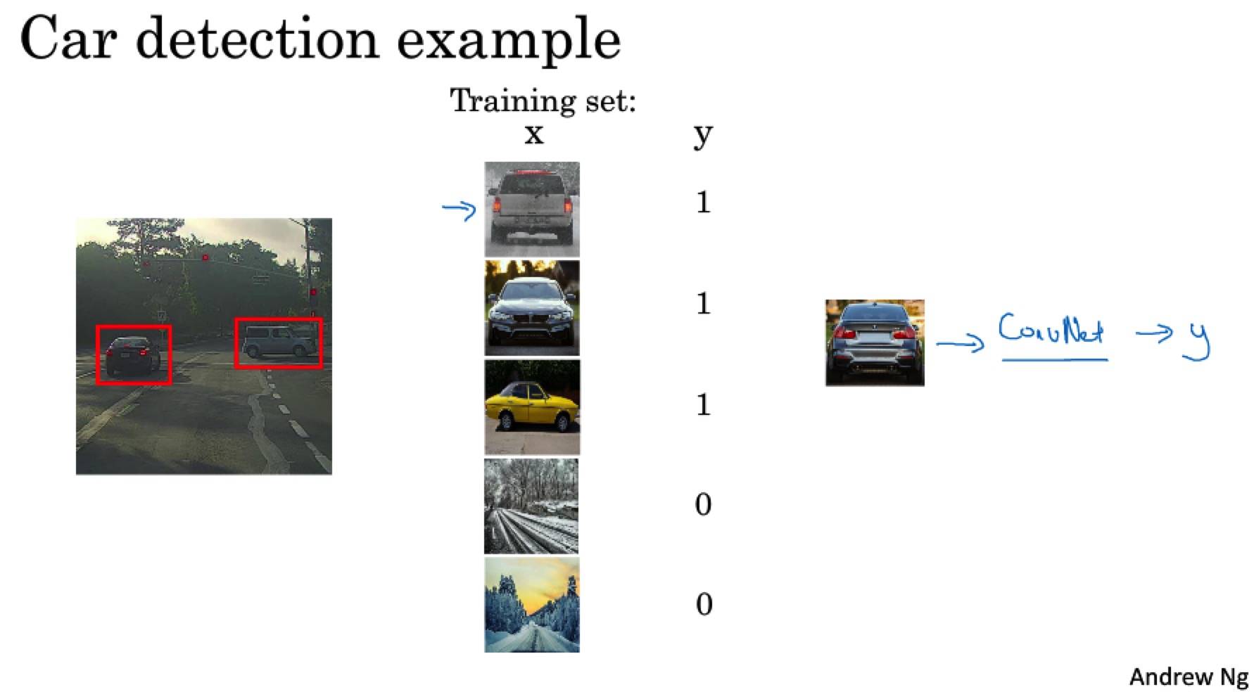
目标监测
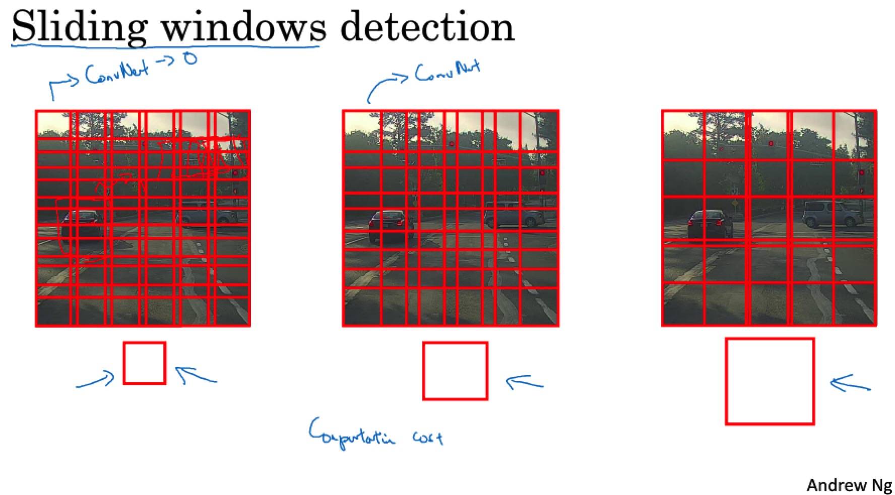
卷积的滑动窗口实现

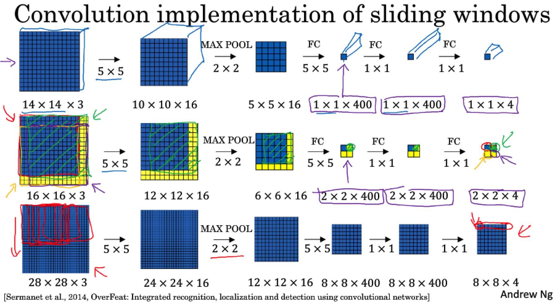
对整张图片进行卷积操作,一次得到所有的预测值。不需要通过连续的卷积操作。
Bounding Box 预测
卷积滑动窗口不能输出最精确的边界框。
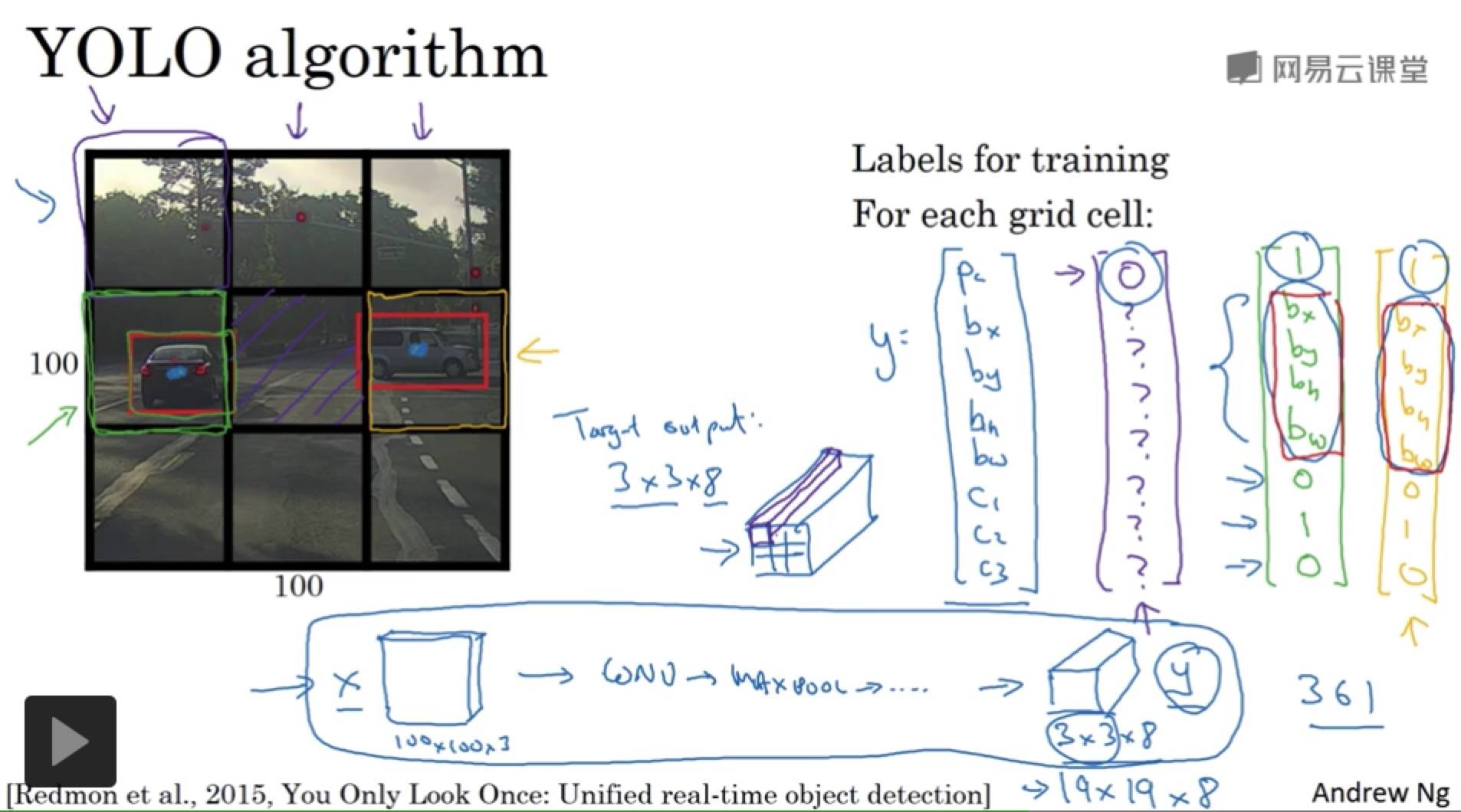
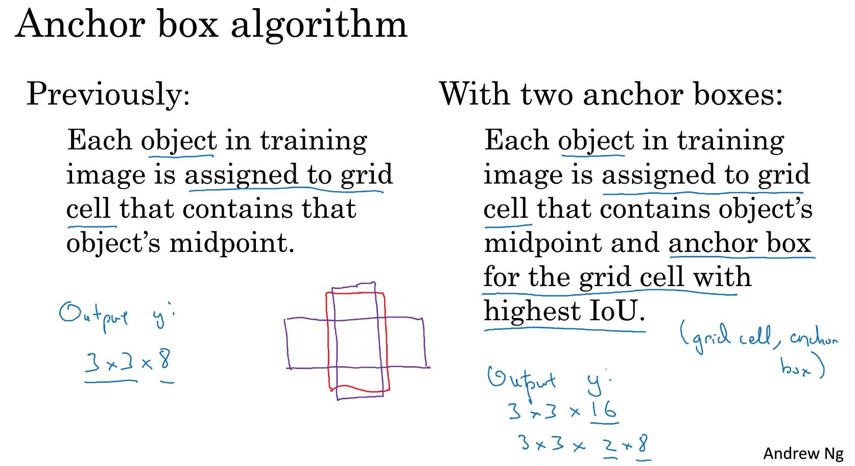
实际中,网格会更精细,多个对象被分配到同一个格子的概率就小很多。
把对象分配到一个格子的过程是,你观察对象的中点,然后将这个对象分配到其中点所在的格子。所以即使对象占多个格子,也只会被分配到其中一个格子。
注意:
- 和分类、定位算法非常类似,能够输出边界框坐标。
- 卷积实现,不需要在每个网格上跑一次算法;单次卷积,有很多共享计算。(YOLO 算法)
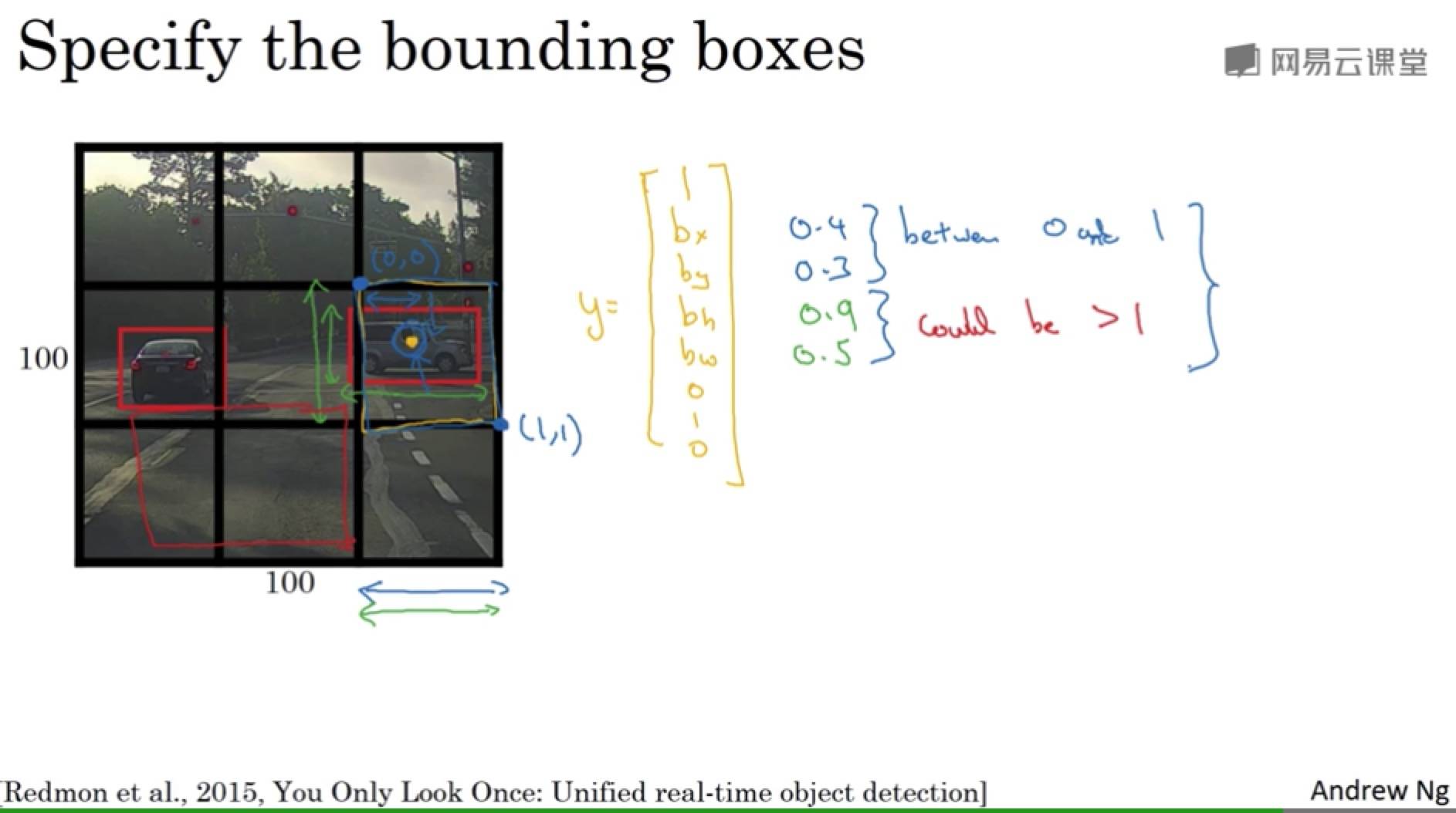
bh, bw 的单位是相对格子尺度的比例
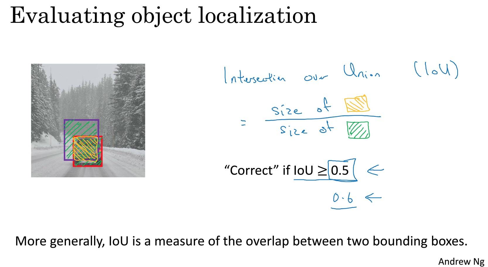
交并比
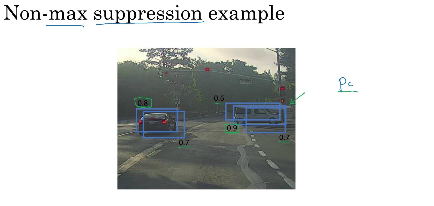
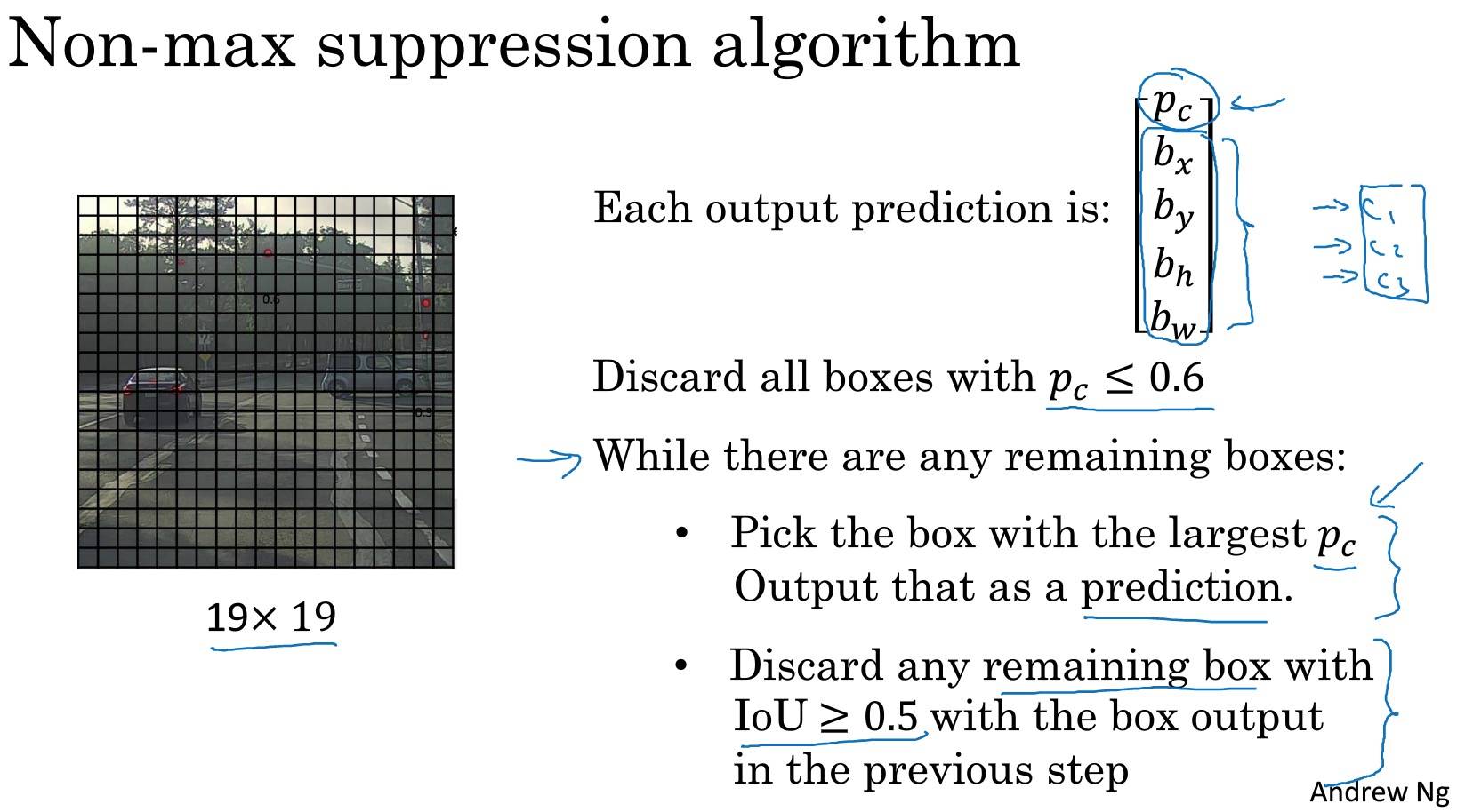
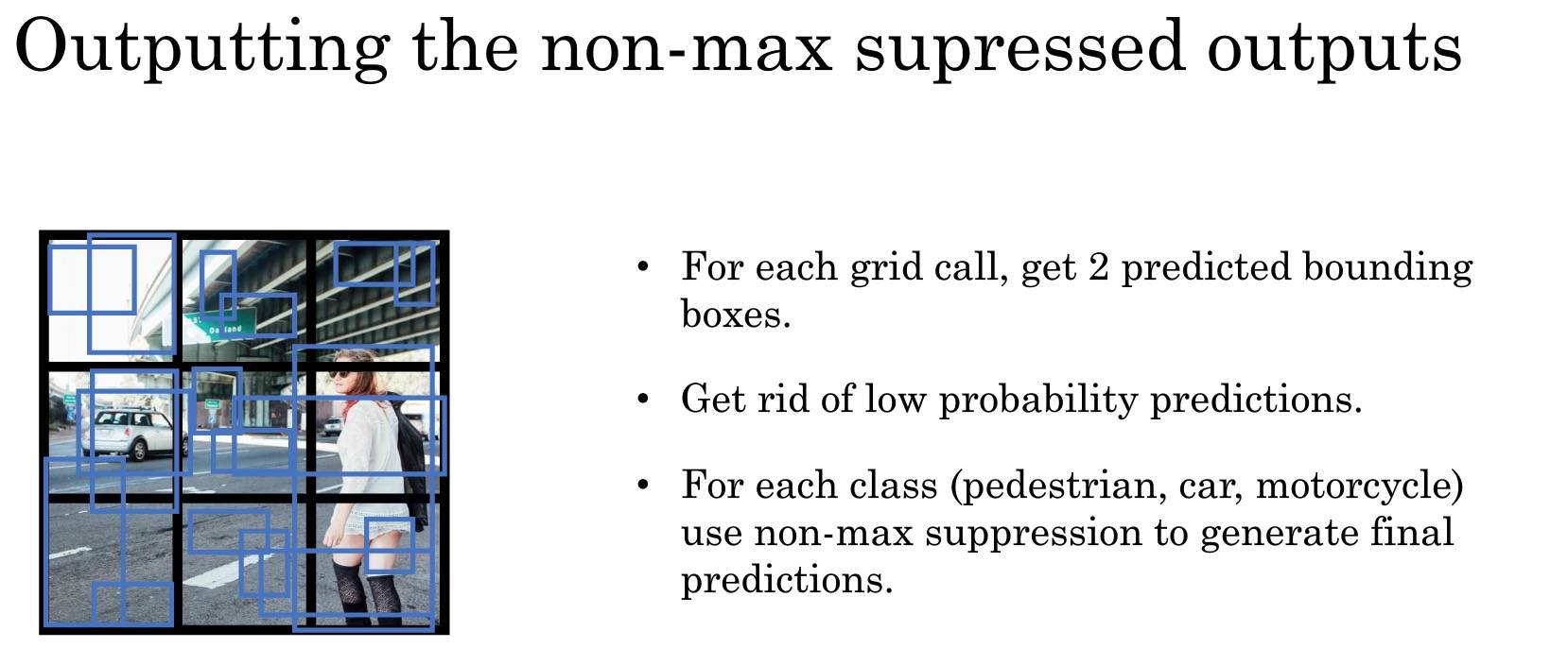
非最大值抑制
确保对每个对象只检测一次,该对象可能有多个。
Anchor Boxes
一个格子检测(有)多个对象(多个物体,对象可能是人、汽车等等),即多个对象中心点在一个格子里。
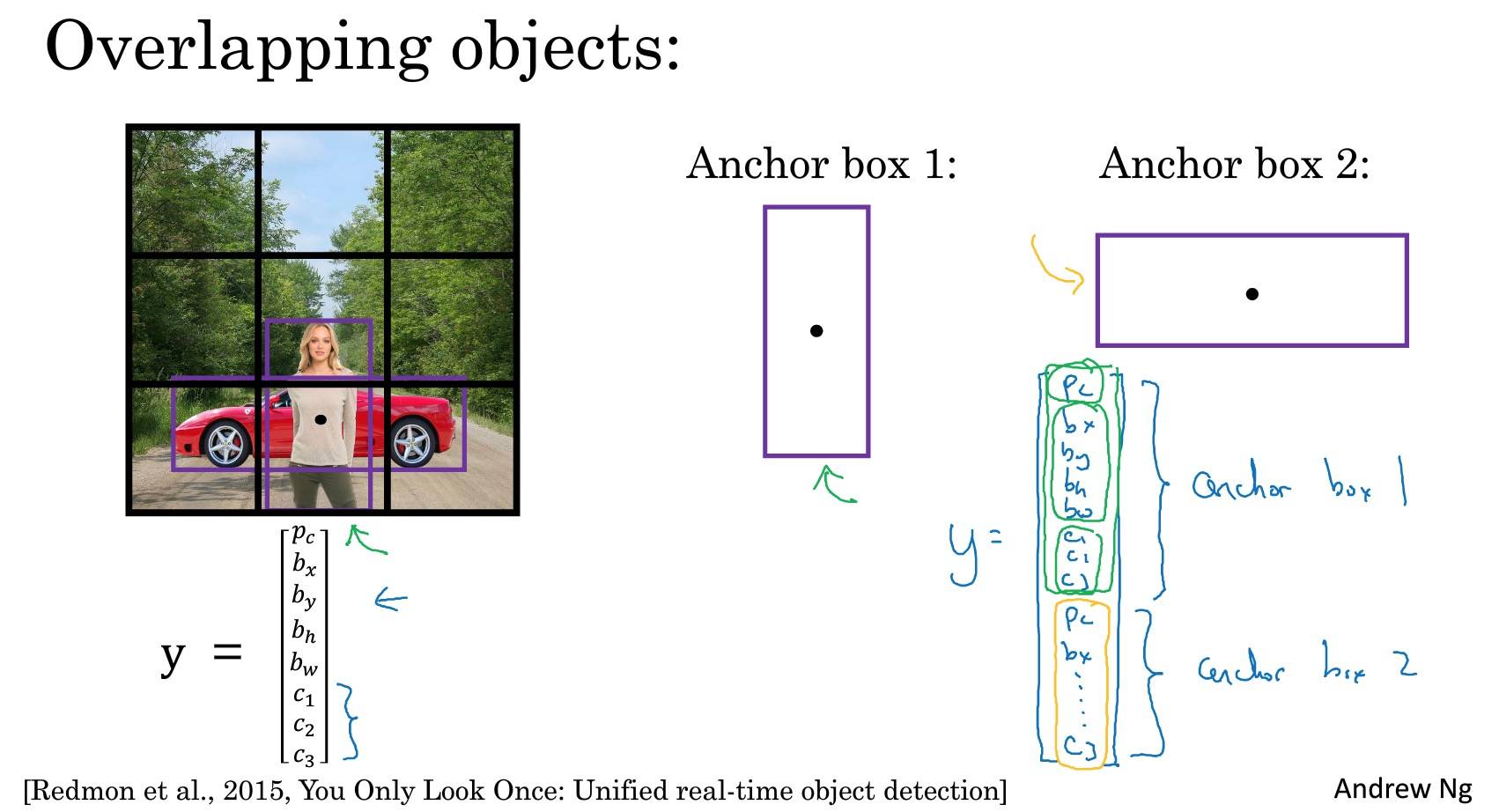

两种情况算法处理不好:
- 同一个格子里有超过 anchor boxes 数量的对象
- 两个对象都分配到一个格子里,并且 anchor box 的形状也一样
Anchor Boxes 能让算法更有针对性,特别是数据集中有一些很高很瘦的对象如行人,或者很矮很胖的对象如汽车。
如何选择 Anchor Box 的形状:
- 一般手工指定 Anchor Box 的形状,选择 5-10 个涵盖要检测对象的各种形状。
- k-means,对两类对象形状聚类,选择最具代表性的一组 Anchor Box,可以代表试图检测 十多个 对象。
这里倒是可以借鉴到 NLP 中的歧义问题里。歧义其实也就是有多个 Anchor Box。
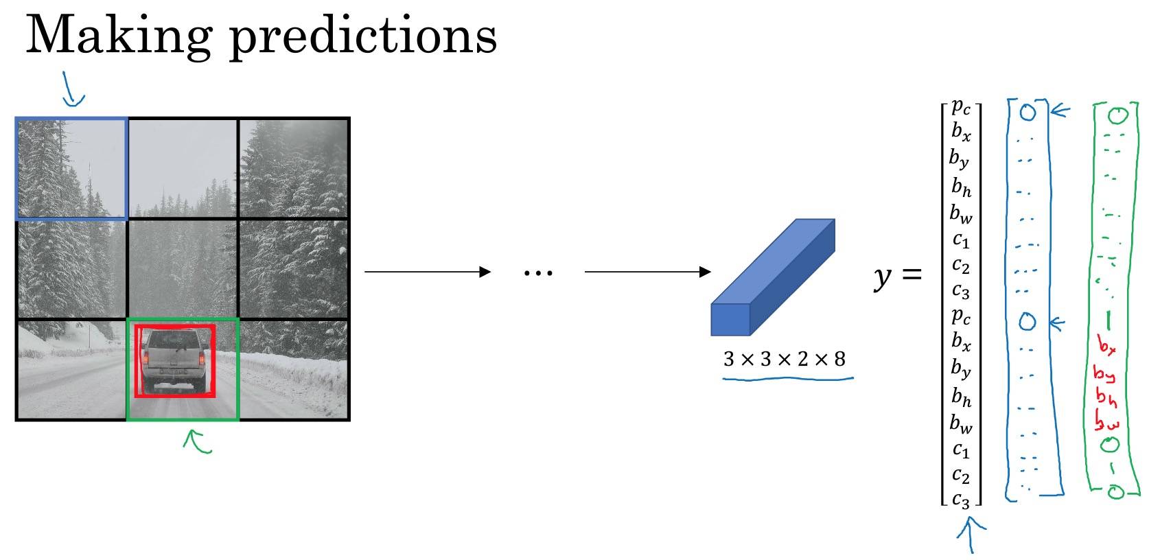
YOLO 算法

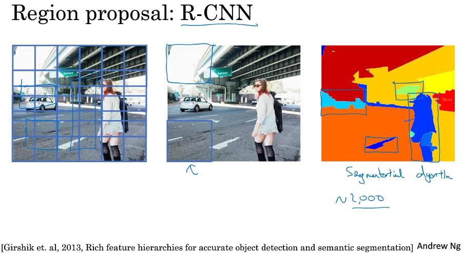
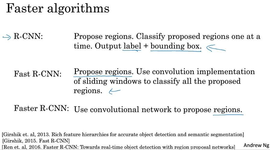
RPN 网络
不再针对每个滑动窗跑检测算法,而是只选择一些窗口,在少数窗口上运行卷积网络分类器。
选出候选区域的方法是:图像分割算法,在每个色块(各种尺寸)上跑分类器。
注意点&Tips
- Summary for YOLO:
- Input image (608, 608, 3)
- The input image goes through a CNN, resulting in a (19,19,5,85) dimensional output.
- After flattening the last two dimensions, the output is a volume of shape (19, 19, 425):
- Each cell in a 19x19 grid over the input image gives 425 numbers.
- 425 = 5 x 85 because each cell contains predictions for 5 boxes, corresponding to 5 anchor boxes, as seen in lecture.
- 85 = 5 + 80 where 5 is because has 5 numbers, and and 80 is the number of classes we’d like to detect
- You then select only few boxes based on:
- Score-thresholding: throw away boxes that have detected a class with a score less than the threshold
- Non-max suppression: Compute the Intersection over Union and avoid selecting overlapping boxes
- This gives you YOLO’s final output.
Week4 特殊应用:人脸识别和神经风格转换
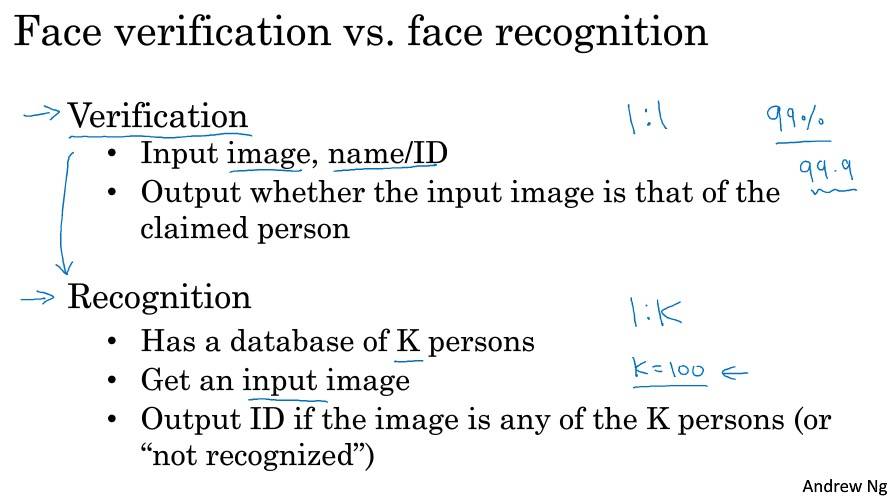
什么是人脸识别?
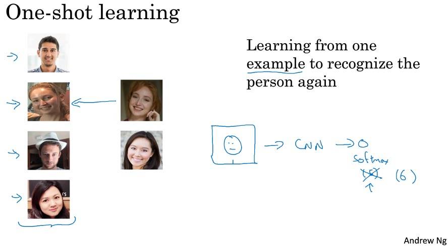
One-Short 学习

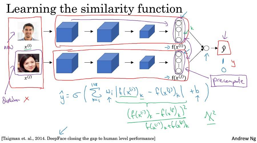
Siamese 网络
[Taigman et. al., 2014. DeepFace closing the gap to human level performance]
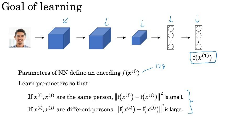
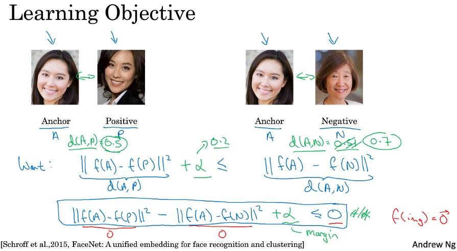
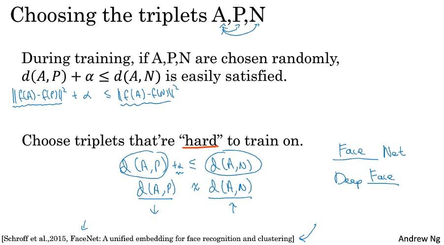
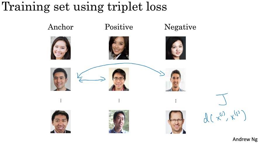
Triplet 损失

面部验证与二分类
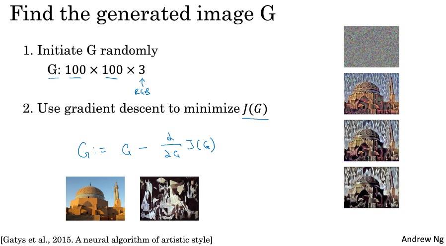
什么是神经风格转移
Content + Style = Generated
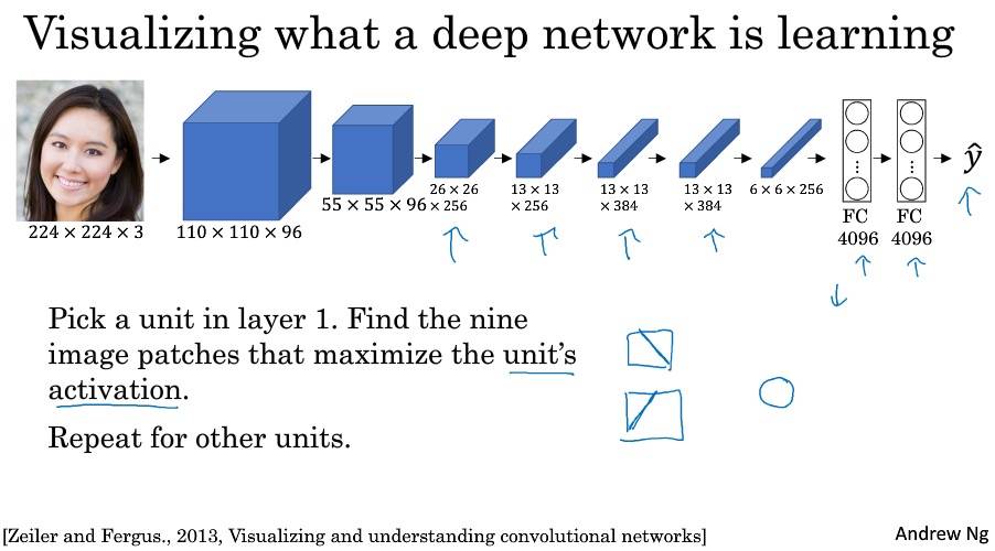
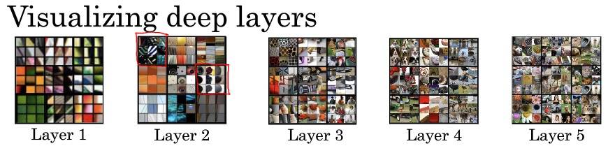
深度卷积网络在学什么?
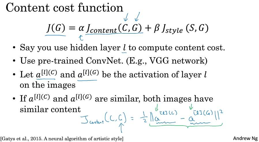
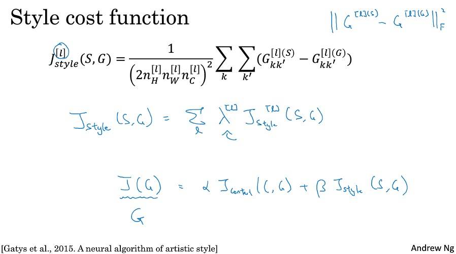
代价函数
J(G) = αJcontent(C,G) + βJstyle(S, G)
内容代价函数
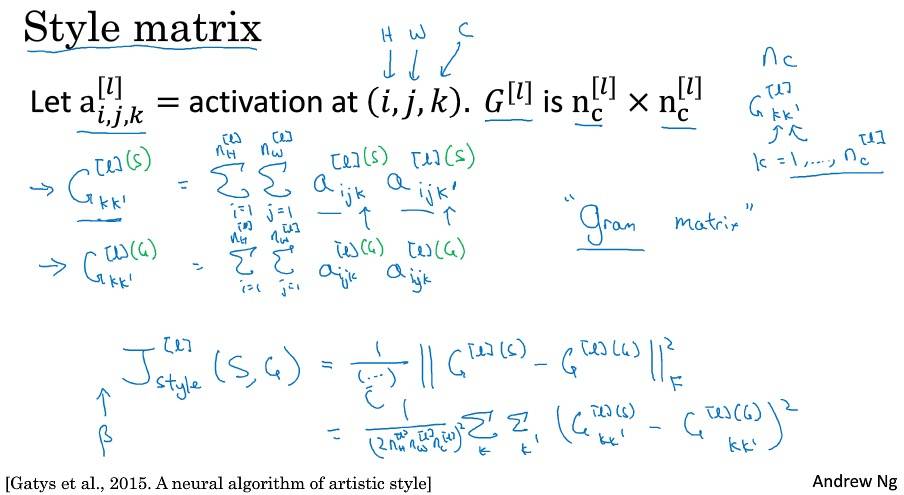
风格代价函数
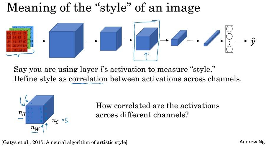
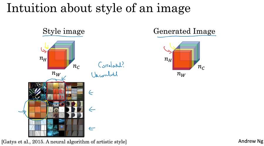
相关系数描述的是在该通道颜色下,出现垂直纹理的概率,即同时出现该通道颜色和垂直纹理或同时不出现的概率。推广而言,就是不同特征在图片不同位置同时出现或不同时出现的概率。
在通道之间,使用相关系数描述通道的风格,就能够测量出生成图片和原始图片风格的相似程度。
如果放在 NLP 中,风格特征是不是就是不同特征词相类似的分布?但是图片本来就是由多通道叠加起来构成的,通道之间关系自然就是其 “风格”,但 NLP 却不具备这样的特征。
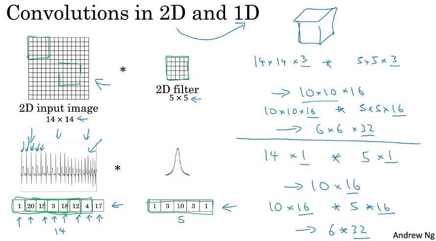
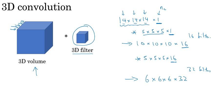
一维到三维推广
注意点&Tips
- Face Recognition
- Face verification solves an easier 1:1 matching problem; face recognition addresses a harder 1:K matching problem.
- The triplet loss is an effective loss function for training a neural network to learn an encoding of a face image.
- The same encoding can be used for verification and recognition. Measuring distances (
np.linalg.norm) between two images’ encodings allows you to determine whether they are pictures of the same person.
- Neural Style Transfer
-
Content Cost
-
lower-level features such as edges and simple textures, and the later (deeper) layers tend to detect higher-level features such as more complex textures as well as object classes.
-
The content cost takes a hidden layer activation of the neural network, and measures how different and are.
-
When we minimize the content cost later, this will help make sure has similar content as .
-
In order to compute the cost , it might also be convenient to unroll these 3D volumes into a 2D matrix:

-
-
Style Cost
-
Style matrix is also called a “Gram matrix.” In linear algebra, the Gram matrix G of a set of vectors is the matrix of dot products, whose entries are . In other words, compares how similar is to : If they are highly similar, you would expect them to have a large dot product, and thus for to be large.

The result is a matrix of dimension where is the number of filters. The value measures how similar the activations of filter are to the activations of filter .
One important part of the gram matrix is that the diagonal elements such as also measures how active filter is. For example, suppose filter is detecting vertical textures in the image. Then measures how common vertical textures are in the image as a whole: If is large, this means that the image has a lot of vertical texture.
-
Style cost: After generating the Style matrix (Gram matrix), the goal will be to minimize the distance between the Gram matrix of the “style” image S and that of the “generated” image G.
-
Style weights: We’ll get better results if we “merge” style costs from several different layers.
-
The style of an image can be represented using the Gram matrix of a hidden layer’s activations. However, we get even better results combining this representation from multiple different layers. This is in contrast to the content representation, where usually using just a single hidden layer is sufficient. Minimizing the style cost will cause the image to follow the style of the image .
-
DONOT NEED to generate image completely random. We initialize the “generated” image as a noisy image created from the content_image. By initializing the pixels of the generated image to be mostly noise but still slightly correlated with the content image, this will help the content of the “generated” image more rapidly match the content of the “content” image.
-
-
Summary
It uses representations (hidden layer activations) based on a pretrained ConvNet. The content cost function is computed using one hidden layer’s activations. The style cost function for one layer is computed using the Gram matrix of that layer’s activations. The overall style cost function is obtained using several hidden layers.
-